Introduction
“You see, Vergon 6 was once filled with the super-dense substance known as dark matter, each pound of which weighs over 10,000 pounds.” — Futurama, S1E4
Numbat is a statically typed programming language for scientific computations with first class support for physical dimensions and units.
You can use it for simple mathematical computations:
>>> 1920/16*9

    = 1080

>>> 2^32

    = 4294967296

>>> sqrt(1.4^2 + 1.5^2) * cos(pi/3)^2

    = 0.512957
The real strength of Numbat, however, is to perform calculations with physical units:
>>> 8 km / (1 h + 25 min)

  8 kilometer / (1 hour + 25 minute)

    = 5.64706 km/h    [Velocity]

>>> 140 € -> GBP

  140 euro ➞ british_pound

    = 120.768 £    [Money]

>>> atan2(30 cm, 1 m) -> deg

  atan2(30 centimeter, 1 meter) ➞ degree

    = 16.6992°

>>> let ω = 2π c / 660 nm

  let ω: Frequency = 2 π × c / 660 nanometer

>>> ℏ ω -> eV

  ℏ × ω ➞ electronvolt

    = 1.87855 eV    [Energy]
Read the tutorial to learn more about the language or look at some example programs. You can also jump directly to the syntax reference.
Tutorial
In this tutorial, you will use Numbat to calculate how many bananas you would need to power a house. This is based on an article in the great what if? series by the author of the xkcd comics.

Bananas contain potassium. In its natural form, potassium contains a tiny fraction (0.0117%)
of the isotope 40K, which is radioactive. The idea is to
use the radioactive decay energy as a power source. Open an interactive Numbat session by
typing numbat in your favorite terminal emulator. We start by entering a few facts about
potassium-40:
let halflife = 1.25 billion years
let occurrence = 0.0117%
let molar_mass = 40 g / mol
New constants are introduced with the let keyword. We
define these physical quantities with their respective physical units (years,
percent, g / mol) in order to profit from Numbat’s unit-safety and unit-conversion
features later on.
Our first goal is to compute the radioactivity of natural potassium. Instead of dealing with the
half-life, we want to know the decay rate. When entering the following computation, you can try
Numbat’s auto-completion functionality. Instead of typing out halflife, just type half and press
Tab.
let decay_rate = ln(2) / halflife
As you can see, we can use typical mathematical functions such as the
natural logarithm ln. Next, we are interested how much radioactivity comes from a certain
mass of potassium:
let radioactivity =
    N_A * occurrence * decay_rate / molar_mass -> Bq / g
The -> Bq / g part at the end converts the expression to Becquerel per gram. If you type
in radioactivity, you should see a result of roughly 31 Bq / g, i.e. 31 radioactive
decays per second, per gram of potassium.
The unit conversion also serves another purpose. If anything would be wrong with our calculation at the units-level, Numbat would detect that and show an error. Unit safety is a powerful concept not just because you can eliminate an entire category of errors, but also because it makes your computations more readable.
We are interested in the radioactivity of bananas, so we first introduce a new (base) unit:
unit banana
This lets us write readable code like
let potassium_per_banana = 451 mg / banana

let radioactivity_banana = potassium_per_banana * radioactivity -> Bq / banana
and should give you a result of roughly 14 Bq / banana. Adding unit conversions at the end
of unit definitions is one way to enforce unit safety. An even more powerful way to do this
is to add type annotations: For example, to define the decay energy for a single
potassium-40 atom,
you can optionally add a : Energy annotation that will be enforced by Numbat:
let energy_per_decay: Energy = 11% × 1.5 MeV + 89% × 1.3 MeV
This also works with custom units since Numbat adds new physical dimensions (types) implicitly:
let power_per_banana: Power / Banana = radioactivity_banana * energy_per_decay
You’ll also notice that types can be combined via mathematical operators such as / in this example.
How many bananas we need to power a household is going to depend on the average power consumption of that household. So we are defining a simple function
fn household_power(annual_consumption: Energy) -> Power = annual_consumption / year
This allows us to finally answer the original question (for a typical US household in 2021)
household_power(10000 kWh) / power_per_banana
This should give you a result of roughly 4×10¹⁴ bananas1.

Attribution
The images in this tutorial are from https://what-if.xkcd.com/158/. They are licensed under the Creative Commons Attribution-NonCommercial 2.5 License. Details and usage notes can be found at https://xkcd.com/license.html.
-
Interestingly, the what if article comes up with a result of 300 quadrillion bananas, or 3 × 10¹⁷. This is a factor of 1000 higher. This seems like a mistake in the original source. All of our other intermediate results are consistent with what has been computed in the original article. ↩
Examples
This chapter shows some exemplary Numbat programs from various disciplines and sciences.
Acidity
# Compute the pH (acidity) of a solution based
# on the activity of hydrogen ions
#
# https://en.wikipedia.org/wiki/PH

fn pH_acidity(activity_hplus: Molarity) -> Scalar =
    - log10(activity_hplus / (mol / L))

print(pH_acidity(5e-6 mol / L))
Barometric formula
# This script calculates the air pressure at a specified
# height above sea level using the barometric formula.

let p0: Pressure = 1 atm
let t0: Temperature = 288.15 K

dimension TemperatureGradient = Temperature / Length
let lapse_rate: TemperatureGradient = 0.65 K / 100 m

fn air_pressure(height: Length) -> Pressure =
    p0 · (1 - lapse_rate · height / t0)^5.255

print("Air pressure 1500 m above sea level: {air_pressure(1500 m) -> hPa}")
Body mass index
# This script calculates the Body Mass Index (BMI) based on
# the provided mass and height values.

unit BMI: Mass / Length^2 = kg / m^2

fn body_mass_index(mass: Mass, height: Length) =
    mass / height² -> BMI

print(body_mass_index(70 kg, 1.75 m))
Factorial
# Naive factorial implementation to showcase recursive
# functions and conditionals.

fn factorial(n) =
  if n < 1
    then 1
    else n × factorial(n - 1)

# Compare result with the builtin factorial operator
assert_eq(factorial(10), 10!)
Flow rate in a pipe
# This script calculates and prints the flow rate in a pipe
# using the Hagen-Poiseuille equation. It assumes the dynamic
# viscosity of water and allows for inputs of pipe radius,
# pipe length, and pressure difference.

let μ_water: DynamicViscosity = 1 mPa·s

fn flow_rate(radius: Length, length: Length, Δp: Pressure) -> FlowRate =
    π × radius^4 × Δp / (8 μ_water × length)

let pipe_radius = 1 cm
let pipe_length = 10 m
let Δp = 0.1 bar

let Q = flow_rate(pipe_radius, pipe_length, Δp)
print("Flow rate: {Q -> L/s}")
Medication dosage
# This script calculates the total daily dose and per intake
# dose of a medication based on a person's body weight.

@aliases(takings)
unit taking

let body_weight = 75 kg
let dosage = (60 mg / kg) / day
let frequency = 3 takings / day

let total_daily_dose = dosage * body_weight -> mg / day
print("Total daily dose: {total_daily_dose}")

let single_dose = total_daily_dose / frequency
print("Single dose:      {single_dose}")
Molarity
# This script calculates and prints the molarity of a salt
# water solution, given a fixed mass of salt (NaCl) and a
# volume of water.

let molar_mass_NaCl = 58.44 g / mol

fn molarity(mass: Mass, volume: Volume) -> Molarity =
    (mass / molar_mass_NaCl) / volume

let salt_mass = 9 g
let water_volume = 1 L

print(molarity(salt_mass, water_volume) -> mmol / l)
Musical note frequency
# Musical note frequencies in the 12 equal temperament system

let frequency_A4: Frequency = 440 Hz  # the A above middle C, A4

fn note_frequency(n: Scalar) -> Frequency = frequency_A4 * 2^(n / 12)

print("A5: {note_frequency(12)}")  # one octave higher up, 880 Hz
print("E4: {note_frequency(7)}")
print("C4: {note_frequency(-3)}")
Paper sizes
# Compute ISO 216 paper sizes for the A series
#
# https://en.wikipedia.org/wiki/ISO_216

struct PaperSize {
    width: Length,
    height: Length,
}

fn paper_size_A(n: Scalar) -> PaperSize =
  if n == 0
    then
      PaperSize {
        width: 841 mm,
        height: 1189 mm
      }
    else
      PaperSize {
        width: floor_in(mm, paper_size_A(n - 1).height / 2),
        height: paper_size_A(n - 1).width,
      }


fn paper_area(size: PaperSize) -> Area =
    size.width * size.height


fn size_as_string(size: PaperSize) = "{size.width:>4} × {size.height:>5}   {paper_area(size) -> cm²:>6.1f}"
fn row(n) = "A{n:<3}   {size_as_string(paper_size_A(n))}"

print("Name    Width     Height        Area  ")
print("----   -------   --------   ----------")
print(join(map(row, range(0, 10)), "\n"))
Population growth
# Exponential model for population growth

let initial_population = 50_000 people
let growth_rate = 2% per year

fn predict_population(t) =
    initial_population × e^(growth_rate·t) |> round_in(people)

print("Population in  20 years: {predict_population(20 years)}")
print("Population in 100 years: {predict_population(1 century)}")
Recipe
# Scale ingredient quantities based on desired servings.

@aliases(servings)
unit serving

let original_recipe_servings = 2 servings
let desired_servings = 3 servings

fn scale(quantity) =
    quantity × desired_servings / original_recipe_servings

print("Milk:          {scale(500 ml)}")
print("Flour:         {scale(250 g)}")
print("Sugar:         {scale(2 cups)}")
print("Baking powder: {scale(4 tablespoons)}")
Voyager
# How many photons are received per bit transmitted from Voyager 1?
#
# This calculation is adapted from a Physics Stack Exchange answer [1].
#
# [1] https://physics.stackexchange.com/a/816710

# Voyager radio transmission:
let datarate = 160 bps
let f = 8.3 GHz
let P_transmit = 23 W

let ω = 2π f
let λ = c / f

@aliases(photon)
unit photons

let energy_per_photon = ℏ ω / photon

let photon_rate = P_transmit / energy_per_photon -> photons/s

print("Voyager sends data at a rate of {datarate} with {P_transmit}.")
print("At a frequency of {f}, this amounts to {photon_rate:.0e}.")

# Voyager dish antenna:
let d_voyager = 3.7 m

# Voyagers distance to Earth:
let R = 23.5 billion kilometers  # as of 2024

# Diameter of receiver dish:
let d_receiver = 70 m

let irradiance = P_transmit / (4π R²)
let P_received: Power = irradiance × (π d_voyager / λ)² × (π d_receiver² / 4)

print("A {d_receiver} dish on Earth will receive {P_received -> aW:.1f} of power.")

let photon_rate_receiver = P_received / energy_per_photon -> photons/s
let photons_per_bit = photon_rate_receiver / datarate -> photons/bit

print()
print("This corresponds to {photon_rate_receiver}.")
print("Which means {photons_per_bit:.0}.")
XKCD 681
# Gravity wells
#
# https://xkcd.com/681/

use extra::astronomy

fn well_depth(mass: Mass, radius: Length) -> Length =
    G × mass / (g0 × radius) -> km

print("Gravity well depths:")
print("Sun     {well_depth(solar_mass, solar_radius):8.0f}")
print("Earth   {well_depth(earth_mass, earth_radius):8.0f}")
print("Moon    {well_depth(lunar_mass, lunar_radius):8.0f}")
print("Mars    {well_depth(mars_mass,  mars_radius):8.0f}")
print("Jupiter {well_depth(jupiter_mass, jupiter_radius):8.0f}")
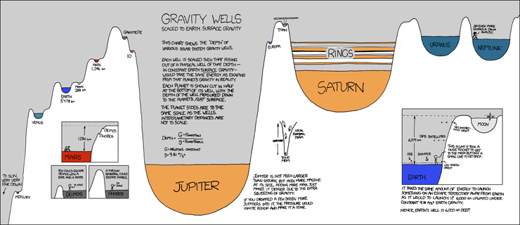
Source: https://xkcd.com/681/
XKCD 687
# Dimensional analysis
#
# https://xkcd.com/687/

let core_pressure = 3.5 million atmospheres
let prius_milage = 50 miles per gallon
let min_width_channel = 21 miles

# Make sure that the result is dimensionless:
let r: Scalar =
    planck_energy / core_pressure × prius_milage / min_width_channel

print("{r} ≈ π ?")
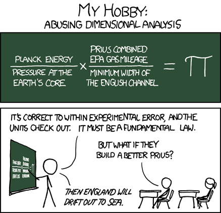
Source: https://xkcd.com/687/
XKCD 2585
# Rounding
#
# https://xkcd.com/2585/

let speed = 17 mph |>
  round_in(meters/sec) |>
  round_in(knots) |>
  round_in(fathoms/sec) |>
  round_in(furlongs/min) |>
  round_in(fathoms/sec) |>
  round_in(kph) |>
  round_in(knots) |>
  round_in(kph) |>
  round_in(furlongs/hour) |>
  round_in(mi/h) |>
  round_in(m/s) |>
  round_in(furlongs/min) |>
  round_in(yards/sec) |>
  round_in(fathoms/sec) |>
  round_in(m/s) |>
  round_in(mph) |>
  round_in(furlongs/min) |>
  round_in(knots) |>
  round_in(yards/sec) |>
  round_in(fathoms/sec) |>
  round_in(knots) |>
  round_in(furlongs/min) |>
  round_in(mph)

print("I can ride my bike at {speed}.")
print("If you round.")
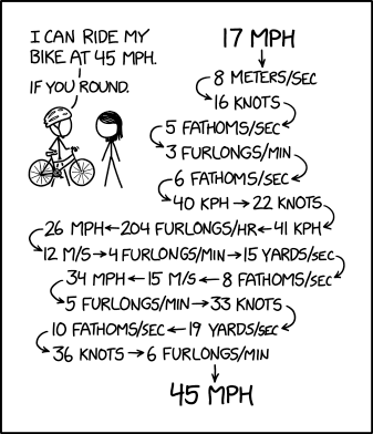
Source: https://xkcd.com/2585/
XKCD 2812
# Solar panel placement
#
# Solar energy tip: To maximize sun exposure, always
# orient your panels downward and install them on the
# surface of the sun.
#
# https://xkcd.com/2812/
#
# [1] https://en.wikipedia.org/wiki/Solar_luminosity
# [2] https://en.wikipedia.org/wiki/Sun

let net_metering_rate = $ 0.20 / kWh
let panel_area = 1 m²
let panel_efficiency = 20 %

fn savings(i: Irradiance) -> Money / Time =
    net_metering_rate × i × panel_area × panel_efficiency -> $/year

print("Option A: On the roof, south facing")

let savings_a = savings(4 kWh/m²/day)

print(savings_a |> round_in($/year))

print()
print("Option B: On the sun, downward facing")

dimension Luminosity = Power

let sun_luminosity: Luminosity = 3.828e26 W  # [1]
let sun_area: Area = 6.09e12 km^2            # [2]

let savings_b = savings(sun_luminosity / sun_area)

print(savings_b |> round_in($/year))
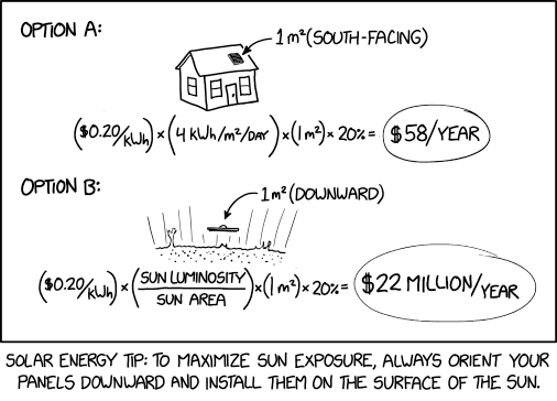
Source: https://xkcd.com/2812/
Basics
This chapter introduces language features that are required to perform basic computations in Numbat or to write small programs.
Number notation
Numbers in Numbat can be written in the following forms:
- Integer notation
1234512_345— with decimal separators
- Floating point notation
0.234.234— without the leading zero
- Scientific notation
1.234e151.234e+151e-91.0e-9
- Non-decimal bases notation
0x2A— Hexadecimal0o52— Octal0b101010— Binary
- Non-finite numbers
NaN— Not a numberinf— Infinity
Convert numbers to other bases
You can use the bin, oct, dec and hex functions to convert numbers to binary, octal, decimal and hexadecimal bases,
respectively. You can call those using hex(2^16 - 1), but they are also available as targets of the conversion operator ->/to,
so you can write expressions like:
Examples:
0xffee -> bin
42 -> oct
2^16 - 1 -> hex

# using 'to':
0xffee to bin
You can also use base(b, n) to convert a number n to base b. Using the reverse function application operator |> you can write
this in a similar style to the previous examples:
273 |> base(3)
144 |> base(12)
Unit notation
Most units can be entered in the same way that they would appear in textbook calculations. They
usually have a long form (meter, degrees, byte, …), a plural form (meters, degrees, bytes),
and a short alias (m, °, B). For a full list of supported units, see
this page.
All SI-accepted units support metric prefixes (mm, cm, km, … or millimeter, centimeter, kilometer, …)
and — where sensible — units allow for binary prefixes (MiB, GiB, … or mebibyte, gibibyte, …). Note
that the short-form prefixes can only be used with the short version of the unit, and vice versa (that is: kmeter and kilom are not allowed, only km and kilometer).
Units can be combined using mathematical operations such as multiplication, division and exponentiation: kg * m/s^2, km/h, m², meter per second.
The following snippet shows various styles of entering units:
2 min + 1 s
150 cm
sin(30°)
50 mph
6 MiB

2 minutes + 1 second
150 centimeters
sin(30 degrees)
50 miles per hour
6 mebibyte
Note that Numbat also allows you to define new units.
Operations and precedence
Numbat operators and other language constructs, ordered by precedence form high to low:
| Operation / operator | Syntax |
|---|---|
| square, cube, … | x², x³, x⁻¹, … |
| factorials | x!, x!!, x!!!, … |
| exponentiation | x^y, x**y |
| multiplication (implicit) | x y (whitespace) |
| unary negation | -x |
| division | x per y |
| division | x / y, x ÷ y |
| multiplication (explicit) | x * y, x · y, x × y |
| subtraction | x - y |
| addition | x + y |
| comparisons | x < y, x <= y, x ≤ y, … x == y, x != y |
| logical negation | !x |
| logical ‘and’ | x && y |
| logical ‘or’ | x || y |
| unit conversion | x -> y, x → y, x ➞ y, x to y |
| conditionals | if x then y else z |
| reverse function call | x |> f |
Note that implicit multiplication has a higher precedence than division, i.e. 50 cm / 2 m will be parsed as 50 cm / (2 m).
Also, note that per-division has a higher precedence than /-division. This means 1 / meter per second will be parsed as 1 / (meter per second).
If in doubt, you can always look at the pretty-printing output (second line in the snippet below) to make sure that your input was parsed correctly:
>>> 1 / meter per second

  1 / (meter / second)

    = 1 s/m
Constants
New constants can be introduced with the let keyword:
let pipe_radius = 1 cm
let pipe_length = 10 m
let Δp = 0.1 bar
Definitions may contain a type annotation after the identifier (let Δp: Pressure = 0.1 bar). This annotation will be verified by the type checker. For more complex definitions
it can be desirable to add type annotations, as it often improves readability and allows
you to catch potential errors early:
let μ_water: DynamicViscosity = 1 mPa·s
let Q: FlowRate = π × pipe_radius^4 × Δp / (8 μ_water × pipe_length)
Unit conversions
The conversion operator -> attempts to convert the physical quantity on its left hand side to
the unit of the expression on its right hand side. This means that you can write an arbitrary
expression on the right hand side — but only the unit part will be extracted. For example:
# simple unit conversion:
> 120 km/h -> mph

  = 74.5645 mi/h

# expression on the right hand side:
> 120 m^3 -> km * m^2

  = 0.12 m²·km

# convert x1 to the same unit as x2:
> let x1 = 50 km / h
> let x2 = 3 m/s -> x1

  x2 = 10.8 km/h
Conversion functions
The conversion operator -> (or to) can not just be used for unit conversions, but also for other types of conversions.
The way this is set up in Numbat is that you can call x -> f for any function f that takes a single argument of the same type as x.
The following functions are available for this purpose:
# Convert a date and time to a Unix timestamp
now() -> unixtime

# Convert a date and time to a different timezone
now() -> tz("Asia/Kathmandu")

# Convert a duration to years, months, days, hours, minutes, seconds
10 million seconds -> human

# Convert an angle to degrees, minutes, seconds (48° 46′ 32″)
48.7756° -> DMS

# Convert an angle to degrees, decimal minutes (48° 46.536′)
48.7756° -> DM

# Convert a number to its binary representation
42 -> bin

# Convert a number to its octal representation
42 -> oct

# Convert a number to its hexadecimal representation
2^31-1 -> hex

# Convert a code point number to a character
0x2764 -> chr

# Convert a character to a code point number
"❤" -> ord

# Convert a string to upper/lower case
"numbat is awesome" -> uppercase
"vier bis elf weiße Querbänder" -> lowercase
Note that the tz(…) call above returns a function, i.e. the right hand side of
the conversion operator is still a function.
Function definitions
Numbat comes with a large number of predefined functions, but
it is also possible to add new functions. A function definition is introduced with
the fn keyword:
fn max_distance(v: Velocity, θ: Angle) -> Length = v² · sin(2 θ) / g0
This exemplary function computes the maximum distance of a projectile under the
influence of Earths gravity. It takes two parameters (the initial velocity v and
the launch angle θ), which are both annotated with their corresponding physical
dimension (their type). The function returns a distance, and so the return type
is specified as Length.
Type inference
Numbat has a powerful type inference system, which is able to infer missing types
when they are not explicitly specified. For example, consider the following function
definition for the braking distance of a car, given its velocity v:
fn braking_distance(v) = v t_reaction + v² / 2 µ g0
  where t_reaction = 1 s # driver reaction time
    and µ = 0.7          # coefficient of friction
If you enter this function into the Numbat REPL, you will see that all types are filled in automatically:
fn braking_distance(v: Velocity) -> Length = v × t_reaction + (v² / (2 µ × g0))
  where t_reaction: Time = 1 second
    and µ: Scalar = 0.7
In particular, note that the type of the function argument v is correctly inferred as
Velocity, and the return type is Length.
Note: This is possible because the types of
t_reaction,µ, andg0(gravitational acceleration) are known. The+operator imposes a constraint on the types: two quantities can only be added if their physical dimension is the same. The type inference algorithm records constraints like this, and then tries to find a solution that satisfies all of them. In this case, only a single equation needs to be solved:type(v) × type(t_reaction) = type(v)² / (type(µ) × type(g0) ) type(v) × Time = type(v)² / ( 1 × Length / Time²)which has the solution
type(v) = Length / Time = Velocity. Note that this also works if there are multiple constraints on the types. In fact, type inference is always decidable.
The fact that it is possible to omit type annotations does not mean that it is always a good idea to do so. Type annotations can help to make the code more readable and can also help to catch errors earlier.
In some cases, type inference will also lead to function types that are overly generic. For example, consider the following function to compute the kinetic energy of a massive object in motion:
fn kinetic_energy(mass, speed) = 1/2 * mass * speed^2
In the absence of any type annotations, this function has an overly generic type where
mass and speed can have arbitrary dimensions (but the return type is constrained
accordingly):
fn kinetic_energy<A: Dim, B: Dim>(mass: A, speed: B) -> A × B² = …
In this example, it would be better to specify the types of mass and speed
explicitly (Mass, Velocity). The return type can then be inferred (Energy).
It is still valuable to specify it explicitly, in order to ensure there are no
mistakes in the function implementation.
Generic functions
Sometimes it is useful to write generic functions. For example, consider
max(a, b) — a function that returns the larger of the two arguments. We might
want to use that function with dimensionful arguments such as max(1 m, 1 yd).
To define such a generic function, you can introduce type parameters in angle
brackets:
fn max<D: Dim>(a: D, b: D) -> D =
  if a > b then a else b
This function signature tells us that max takes two arguments of arbitrary
dimension type D (but they need to match!), and returns a quantity of the same
type D. The D: Dim syntax is a type constraint (or bound) that ensures that
D is a dimension type (Scalar, Length, Velocity, etc), and not something
like Bool or DateTime.
Note that you can perform the usual operations with (dimension) type parameters, such as multiplying / dividing them with other types, or raising to rational powers. For example, consider this cube-root function
fn cube_root<T>(x: T^3) -> T = x^(1/3)
that can be called with a scalar (cube_root(8) == 2) or a dimensionful
argument (cube_root(1 liter) == 10 cm).
Note: cube_root can also be defined as fn cube_root<T>(x: T) -> T^(1/3),
which is equivalent to the definition above.
Functions can also be generic over all types, not just dimension types. In this case, no type constraints are needed. For example:
fn second_element<A>(xs: List<A>) -> A =
  head(tail(xs))

second_element([10 cm, 2 m, 3 inch]) # returns 2 m
second_element(["a", "b", "c"])      # returns "b"
Note that the type annotations for all examples in this section are optional and can also be inferred.
Recursive functions
It is also possible to define recursive functions. For example, a naive recursive implementation to compute Fibonacci numbers in Numbat looks like this:
fn fib(n) =
  if n ≤ 2
    then 1
    else fib(n - 2) + fib(n - 1)
Conditionals
Numbat has if-then-else conditional expressions with the following
syntax
if <cond> then <expr1> else <expr2>
where <cond> is a condition that evaluates to a Boolean value, like
3 ft < 3 m. The types of <expr1> and <expr2> need to match.
For example, you can defined a simple step function using
fn step(x) = if x < 0 then 0 else 1
Lists
Numbat has a built-in data type for lists. The elements can be of any type, including other lists.
Lists can be created using the […] syntax. For example:
[30 cm, 110 cm, 2 m]
["a", "b", "c"]
[[1, 2], [3, 4]]
The type of a list is written as List<T>, where T is the type of the elements. The types of the lists
above are List<Length>, List<String>, and List<List<Scalar>>, respectively.
The standard library provides a number of functions to work with lists. Some useful things to do with lists are:
# Get the length of a list
len([1, 2, 3])  # returns 3

# Sum all elements of a list:
sum([30 cm, 130 cm, 2 m])  # returns 360 cm

# Get the average of a list:
mean([30 cm, 130 cm, 2 m])  # returns 120 cm

# Filter a list:
filter(is_finite, [20 cm, inf, 1 m])  # returns [20 cm, 1 m]

# Map a function over a list:
map(sqr, [10 cm, 2 m])  # returns [100 cm², 4 m²]

# Generate a range of numbers:
range(1, 5)  # returns [1, 2, 3, 4, 5]

# Generate a list of evenly spaced quantities:
linspace(0 m, 1 m, 5)  # returns [0 m, 0.25 m, 0.5 m, 0.75 m, 1 m]
Structs
Numbat has compound data structures in the form of structs:
struct Vector {
  x: Length,
  y: Length,
}

let origin   = Vector { x: 0 m, y: 0 m }
let position = Vector { x: 6 m, y: 8 m }

# A function with a struct as a parameter
fn euclidean_distance(a: Vector, b: Vector) =
  sqrt((a.x - b.x)² + (a.y - b.y)²)

assert_eq(euclidean_distance(origin, position), 10 m)

# Struct fields can be accessed using `.field` notation
let x = position.x
Date and time
Numbat supports date and time handling based on the proleptic Gregorian calendar, which is the (usual) Gregorian calendar extended to dates before its introduction in 1582.
A few examples of useful operations that can be performed on dates and times:
# How many days are left until September 1st?
date("2024-11-01") - today() -> days

# What time is it in Nepal right now?
now() -> tz("Asia/Kathmandu")  # use tab completion to find time zone names

# What is the local time when it is 2024-11-01 12:30:00 in Australia?
datetime("2024-11-01 12:30:00 Australia/Sydney") -> local

# Which date was 1 million seconds ago?
now() - 1 million seconds

# Which date is 40 days from now?
calendar_add(now(), 40 days)

# Which weekday was the 1st day of this century?
date("2000-01-01") -> weekday

# What is the current UNIX timestamp?
now() -> unixtime

# What is the date corresponding to a given UNIX timestamp?
from_unixtime(1707568901)

# How long are one million seconds in years, months, days, hours, minutes, seconds?
1 million seconds -> human
Date and time arithmetic
The following operations are supported for DateTime objects:
| Left | Operator | Right | Result |
|---|---|---|---|
DateTime | - | DateTime | Duration between the two dates as a Time. In seconds, by default. Use normal conversion for other time units. |
DateTime | + | Time | New DateTime by adding the duration to the date |
DateTime | - | Time | New DateTime by subtracting the duration from the date |
DateTime | -> | tz("…") | Converts the datetime to the specified time zone. Note that you can use tab-completion for time zone names. |
Warning: You can directly add days, months and years to a given date (now() + 3 months), but note that the result might not be what you expect.
The unit day is defined as having a length of 24 hours. But due to daylight
saving time, days can be shorter or longer than that. A month is defined
as 1/12 of a year, but calendar months have varying lengths. And a year
is defined as the average length of a
tropical year. But a calendar
year can have 365 or 366 days, depending on whether it is a leap year or not.
If you want to take all of these factors into account, you should use the calendar_add/calendar_sub functions instead of directly adding or
subtracting days, months, or years.
Date, time, and duration functions
The following functions are available for date and time handling:
now() -> DateTime: Returns the current date and time.today() -> DateTime: Returns the current date at midnight (in the local time).datetime(input: String) -> DateTime: Parses a string (date and time) into aDateTimeobject.date(input: String) -> DateTime: Parses a string (only date) into aDateTimeobject.time(input: String) -> DateTime: Parses a string (only time) into aDateTimeobject.format_datetime(format: String, dt: DateTime) -> String: Formats aDateTimeobject as a string. See this page for possible format specifiers.tz(tz: String) -> Fn[(DateTime) -> DateTime]: Returns a timezone conversion function, typically used with the conversion operator (datetime -> tz("Europe/Berlin"))local(dt: DateTime) -> DateTime: Timezone conversion function targeting the users local timezone (datetime -> local)get_local_timezone() -> String: Returns the users local timezoneunixtime(dt: DateTime) -> Scalar: Converts aDateTimeto a UNIX timestamp.from_unixtime(ut: Scalar) -> DateTime: Converts a UNIX timestamp to aDateTimeobject.calendar_add(dt: DateTime, span: Time): Add a span of time to aDateTimeobject, taking proper calendar arithmetic into accound.calendar_sub(dt: DateTime, span: Time): Subtract a span of time from aDateTimeobject, taking proper calendar arithmetic into accound.weekday(dt: DateTime) -> String: Returns the weekday of aDateTimeobject as a string.human(duration: Time) -> String: Converts aTimeto a human-readable string in days, hours, minutes and seconds.julian_date(dt: DateTime) -> Scalar: Convert aDateTimeto a Julian date.
Date time formats
The following formats are supported by datetime. UTC offsets are mandatory for the RFC 3339 and
RFC 2822 formats. The other formats can optionally include a time zone name or UTC offset. If no time
zone is specified, the local time zone is used.
| Format | Examples |
|---|---|
| RFC 3339 | 2024-02-10T12:30:00Z2024-02-10T06:30:00-06:00 |
| RFC 2822 | Sat, 10 Feb 2024 12:30:00 ZSat, 10 Feb 2024 06:30:00 -0600 |
%Y-%m-%d %H:%M:%S%.f | 2024-02-10 12:30:002024-02-10 06:30:00 -06002024-02-10 07:30:00 US/Eastern2024-02-10 12:30:00.123456 |
%Y/%m/%d %H:%M:%S%.f | same, but with / separator |
%Y-%m-%d %H:%M | 2024-02-10 12:302024-02-10 06:30 -06002024-02-10 07:30 US/Eastern |
%Y/%m/%d %H:%M | same, but with / separator |
%Y-%m-%d %I:%M:%S%.f %p | 2024-02-10 12:30:00 PM2024-02-10 06:30:00 AM -06002024-02-10 07:30:00 AM US/Eastern2024-02-10 12:30:00.123456 PM |
%Y/%m/%d %I:%M:%S%.f %p | same, but with / separator |
%Y-%m-%d %I:%M %p | 2024-02-10 12:30 PM2024-02-10 06:30 AM -06002024-02-10 07:30 AM US/Eastern |
%Y/%m/%d %I:%M %p | same, but with / separator |
The date function supports the following formats. It returns a DateTime object with the time set to midnight in the
specified timezone (or the local timezone if no timezone is specified).
| Format | Examples |
|---|---|
%Y-%m-%d | 2024-02-102024-02-10 +01002024-02-10 Europe/Berlin |
%Y/%m/%d | 2024/02/102024/02/10 +01002024/02/10 Europe/Berlin |
The time function supports the following formats. It returns a DateTime object with the date set to the current date.
If no timezone is specified, the local timezone is used.
| Format | Examples |
|---|---|
%H:%M:%S%.f | 12:30:0006:30:00 -060007:30:00 US/Eastern12:30:00.123456 |
%H:%M | 12:3006:30 -060007:30 US/Eastern |
%I:%M:%S%.f %p | 12:30:00 PM06:30:00 AM -060007:30:00 AM US/Eastern12:30:00.123456 PM |
%I:%M %p | 12:30 PM06:30 AM -060007:30 AM US/Eastern |
Printing, testing, debugging
Printing
Numbat has a builtin print procedure that can be used to print the value of an expression:
print(2 km/h)
print(3 ft < 1 m)
You can also print out simple messages as strings. This is particularly useful when combined with string interpolation to print results of a computation:
let radius: Length = sqrt(footballfield / 4 pi) -> meter
print("A football field would fit on a sphere of radius {radius}")
You can use almost every expression inside a string interpolation field. For example:
print("3² + 4² = {hypot2(3, 4)}²")

let speed = 25 km/h
print("Speed of the bicycle: {speed} ({speed -> mph})")
Format specifiers are also supported in interpolations. For instance:
print("{pi:0.2f}") # Prints "3.14"
For more information on supported format specifiers, please see this page.
Testing
The assert_eq procedure can be used to test for (approximate) equality of two quantities.
This is often useful to make sure that (intermediate) results in longer calculations have
a certain value, e.g. when restructuring the code. The general syntax is
assert_eq(q1, q2)
assert_eq(q1, q2, ε)
where the first version tests for exact equality while the second version tests for approximate equality \( |q_1-q_2| <= \epsilon \) with a specified accuracy of \( \epsilon \). Note that the input quantities are converted to the units of \( \epsilon \) before comparison. For example:
assert_eq(2 + 3, 5)
assert_eq(1 ft × 77 in², 4 gal)

assert_eq(alpha, 1 / 137, 1e-4)
assert_eq(3.3 ft, 1 m, 1 cm)
There is also a plain assert procedure that can test any boolean condition. For example:
assert(1 yard < 1 meter)
assert(str_contains("bar", "foobar"))
A runtime error is thrown if an assertion fails. Otherwise, nothing happens.
Debugging
You can use the builtin type procedure to see the type (or physical dimension) of a quantity:
>>> type(g0)

  Length / Time²

>>> type(2 < 3)

  Bool
Advanced
This chapter covers more advanced topics, like defining custom physical units or new physical dimensions.
Dimension definitions
New (physical) dimensions can be introduced with the dimension keyword. Similar like for units, there are base dimensions (like length, time and mass) and dimensions that are derived from those base dimensions (like momentum, which is mass · length / time). Base dimensions are simply introduced by declaring their name:
dimension Length
dimension Time
dimension Mass
Derived dimensions need to specify their relation to base dimensions (or other derived dimensions). For example:
dimension Velocity = Length / Time
dimension Momentum = Mass * Velocity
dimension Force = Mass * Acceleration = Momentum / Time
dimension Energy = Momentum^2 / Mass = Mass * Velocity^2 = Force * Length
In the definition of Force and Energy, we can see that multiple alternative definitions can be specified. This is entirely optional. When given, the compiler will make sure that all definitions are equivalent.
Unit definitions
New units of measurement can be introduced with the unit keyword. There are two types of units: base units and derived units.
A new base unit can be defined by specifying the physical dimension it represents. For example, in the International System of Units (SI), the second is the base unit for measuring times:
unit second: Time
Here, Time denotes the physical dimension. To learn more, you can read the corresponding chapter. But for now, we can just assume that they are already given.
Derived units are also introduced with the unit keyword. But unlike base units, they are defined through their relation to
other units. For example, a minute can be defined as
unit minute: Time = 60 second
Here, the : Time annotation is optional. If a dimension is specified, it will be used to verify that the right hand side expression (60 second) is indeed of physical dimension Time. This is apparent in this simple example, but can be useful for more complicated unit definitions like
unit farad: Capacitance = ampere^2 second^4 / (kilogram meter^2)
Prefixes
If a unit may be used with metric prefixes such as milli/m, kilo/k or mega/M, we can prepend the unit definition with the @metric_prefixes decorator:
@metric_prefixes
unit second: Time
This allows identifiers such as millisecond to be used in calculations. See the section below how prefixes interact with aliases.
Similarly, if a unit should be prependable with binary (IEC) prefixes such as kibi/Ki, mebi/Mi or gibi/Gi, you can
add the @binary_prefixes decorator. A unit might also allow for both metric and binary prefixes, for example:
@binary_prefixes
@metric_prefixes
unit byte = 8 bit
This allows the usage of both mebibyte (1024² byte) as well as megabyte (1000² byte).
Aliases
It is often useful to define alternative names for a unit. For example, we might want to use the plural form seconds or the commonly
used short version s. We can use the @aliases decorator to specify them:
@metric_prefixes
@aliases(meters, metre, metres, m: short)
unit meter: Length
In addition to the name, we can also specify how aliases interact with prefixes using : long (the default), : short, : both or
: none. The actual unit name (meter) and all long aliases will accept the long version of prefixes (…, milli, kilo, mega, giga, …).
All short aliases (m in the example above) will only accept the respective short versions of the prefixes (…, m, k, M, G, …).
Aliases annotated with : both or : none accept either both long and short prefixes, or none of them.
The unit definition above allows all of following expressions:
millimeter
kilometer

millimeters
kilometers

millimetre
kilometre

millimetres
kilometres

mm
km
...
Ad-hoc units
It is often useful to introduce ‘fictional’ physical units (and dimensions). This comes up frequently when you want to count things. For example:
unit book

@aliases(pages)
unit page

@aliases(words)
unit word

let words_per_book = 500 words/page × 300 pages/book
Note that those base unit definitions will implicitly create new dimensions which are capitalized
versions of the unit names (Book, Page, Word). A definition like unit book is a shorthand
for dimension Book; unit book: Book.
Those units now allow us to count books, pages
and words independently without any risk of mixing them. The words_per_book constant in this
examples has a type of Word / Book.
Another example shows how we introduce a dot unit to do calculations with
screen resolutions:
@aliases(dots)
unit dot

unit dpi = dots / inch

# Note: a `Dot` dimension was implicitly created for us
fn inter_dot_spacing(resolution: Dot / Length) -> Length = 1 dot / resolution

inter_dot_spacing(72 dpi) -> µm  # 353 µm
Syntax overview
# This is a line comment. It can span over
# multiple lines

# 1. Imports

use prelude        # This is not necessary. The 'prelude'
                   # module will always be loaded upon startup

use units::stoney  # Load a specific module

# 2. Numbers

12345       # integer notation
12_345      # optional decimal separators

0.234       # floating point notation
.234        # without the leading zero

1.234e15    # scientific notation
1.234e+15
1e-9
1.0e-9

0x2A        # hexadecimal
0o52        # octal
0b101010    # binary

NaN         # Not a number
inf         # Infinity

# 3. Simple expressions

3 + (4 - 3)       # Addition and subtraction

1920 / 16 * 9     # Multiplication, division
1920 ÷ 16 × 9     # Unicode-style, '·' or '⋅' works as well
2 pi              # Whitespace is implicit multiplication
meter per second  # 'per' keyword can be used for division

2^3               # Exponentiation
2**3              # Python-style
2³                # Unicode exponents
2^-3              # Negative exponents

mod(17, 4)        # Modulo

3 in -> cm        # Unit conversion, can also be → or ➞
3 in to cm        # Unit conversion with the 'to' keyword

cos(pi/3 + pi)    # Call mathematical functions
pi/3 + pi |> cos  # Same, 'arg |> f' is equivalent to 'f(arg)'
                  # The '|>' operator has the lowest precedence
                  # which makes it very useful for interactive
                  # terminals (press up-arrow, and add '|> f')

_                 # Result of last calculation, also 'ans'

# 4. Constants

let n = 4                          # Simple numerical constant
let q1 = 2 m/s                     # Right hand side can be any expression
let q2: Velocity = 2 m/s           # With optional type annotation
let q3: Length / Time = 2 m/s      # more complex type annotation

# 5. Function definitions

fn foo(z: Scalar) -> Scalar = 2 * z + 3                   # A simple function
fn speed(len: Length, dur: Time) -> Velocity = len / dur  # Two parameters
fn my_sqrt<T: Dim>(q: T^2) -> T = q^(1/2)                 # A generic function
fn is_non_negative(x: Scalar) -> Bool = x ≥ 0             # Returns a bool
fn power_4(x: Scalar) = z                                 # A function with local variables
  where y = x * x
    and z = y * y

# 6. Dimension definitions

dimension Fame                            # A new base dimension
dimension Deceleration = Length / Time^2  # A new derived dimension

# 7. Unit definitions

@aliases(quorks)                 # Optional aliases-decorator
unit quork = 0.35 meter          # A new derived unit

@metric_prefixes                 # Optional decorator to allow 'milliclonk', etc.
@aliases(ck: short)              # short aliases can be used with short prefixes (mck)
unit clonk: Time = 0.2 seconds   # Optional type annotation

@metric_prefixes
@aliases(wh: short)
unit warhol: Fame                # New base unit for the "Fame" dimension

unit thing                       # New base unit with automatically generated
                                 # base dimension "Thing"

# 8. Conditionals

fn bump(x: Scalar) -> Scalar =   # The construct 'if <cond> then <expr> else <expr>'
  if x >= 0 && x <= 1            # is an expression, not a statement. It can span
    then 1                       # multiple lines.
    else 0

# 9. Procedures

print(2 kilowarhol)              # Print the value of an expression
print("hello world")             # Print a message
print("value of pi = {pi}")      # String interpolation
print("sqrt(10) = {sqrt(10)}")   # Expressions in string interpolation
print("value of π ≈ {π:.3}")     # Format specifiers

assert(1 yard < 1 meter)         # Assertion

assert_eq(1 ft, 12 in)           # Assert that two quantities are equal
assert_eq(1 yd, 1 m, 10 cm)      # Assert that two quantities are equal, up to
                                 # the given precision
type(2 m/s)                      # Print the type of an expression


# 10. Structs

struct Element {                 # Define a struct
    name: String,
    atomic_number: Scalar,
    density: MassDensity,
}

let hydrogen = Element {         # Instantiate it
    name: "Hydrogen",
    atomic_number: 1,
    density: 0.08988 g/L,
}

hydrogen.density                 # Access the field of a struct
The prelude
Numbat comes with a special module called prelude that is always loaded on
startup (unless --no-prelude is specified on the command line). This module
is split into multiple submodules and sets up a useful default environment with
mathematical functions, constants but also dimension definitions, unit
definitions and physical constants.
You can find the full source code of the standard library on GitHub.
This chapter is a reference to the prelude module.
Predefined functions
See sub-chapters for a list of predefined functions in the standard library.
Mathematical functions
Basics · Transcendental functions · Trigonometry · Statistics · Combinatorics · Random sampling, distributions · Number theory · Numerical methods · Percentage calculations · Geometry · Algebra · Trigonometry (extra)
Basics
Defined in: core::functions
id (Identity function)
Return the input value.
fn id<A>(x: A) -> A
Examples
id(8 kg)

    = 8 kg    [Mass]
abs (Absolute value)
Return the absolute value \( |x| \) of the input. This works for quantities, too: abs(-5 m) = 5 m.
More information here.
fn abs<T: Dim>(x: T) -> T
Examples
abs(-22.2 m)

    = 22.2 m    [Length]
sqrt (Square root)
Return the square root \( \sqrt{x} \) of the input: sqrt(121 m^2) = 11 m.
More information here.
fn sqrt<D: Dim>(x: D^2) -> D
Examples
sqrt(4 are) -> m

    = 20 m    [Length]
cbrt (Cube root)
Return the cube root \( \sqrt[3]{x} \) of the input: cbrt(8 m^3) = 2 m.
More information here.
fn cbrt<D: Dim>(x: D^3) -> D
Examples
cbrt(8 L) -> cm

    = 20.0 cm    [Length]
sqr (Square function)
Return the square of the input, \( x^2 \): sqr(5 m) = 25 m^2.
fn sqr<D: Dim>(x: D) -> D^2
Examples
sqr(7)

    = 49
round (Rounding)
Round to the nearest integer. If the value is half-way between two integers, round away from \( 0 \). See also: round_in.
More information here.
fn round(x: Scalar) -> Scalar
Examples
round(5.5)

    = 6
round(-5.5)

    = -6
round_in (Rounding)
Round to the nearest multiple of base.
fn round_in<D: Dim>(base: D, value: D) -> D
Examples
Round in meters.
round_in(m, 5.3 m)

    = 5 m    [Length]
Round in centimeters.
round_in(cm, 5.3 m)

    = 530 cm    [Length]
floor (Floor function)
Returns the largest integer less than or equal to \( x \). See also: floor_in.
More information here.
fn floor(x: Scalar) -> Scalar
Examples
floor(5.5)

    = 5
floor_in (Floor function)
Returns the largest integer multiple of base less than or equal to value.
fn floor_in<D: Dim>(base: D, value: D) -> D
Examples
Floor in meters.
floor_in(m, 5.7 m)

    = 5 m    [Length]
Floor in centimeters.
floor_in(cm, 5.7 m)

    = 570 cm    [Length]
ceil (Ceil function)
Returns the smallest integer greater than or equal to \( x \). See also: ceil_in.
More information here.
fn ceil(x: Scalar) -> Scalar
Examples
ceil(5.5)

    = 6
ceil_in (Ceil function)
Returns the smallest integer multiple of base greater than or equal to value.
fn ceil_in<D: Dim>(base: D, value: D) -> D
Examples
Ceil in meters.
ceil_in(m, 5.3 m)

    = 6 m    [Length]
Ceil in centimeters.
ceil_in(cm, 5.3 m)

    = 530 cm    [Length]
trunc (Truncation)
Returns the integer part of \( x \). Non-integer numbers are always truncated towards zero. See also: trunc_in.
More information here.
fn trunc(x: Scalar) -> Scalar
Examples
trunc(5.5)

    = 5
trunc(-5.5)

    = -5
trunc_in (Truncation)
Truncates to an integer multiple of base (towards zero).
fn trunc_in<D: Dim>(base: D, value: D) -> D
Examples
Truncate in meters.
trunc_in(m, 5.7 m)

    = 5 m    [Length]
Truncate in centimeters.
trunc_in(cm, 5.7 m)

    = 570 cm    [Length]
fract (Fractional part)
Returns the fractional part of \( x \), i.e. the remainder when divided by 1.
If \( x < 0 \), then so will be fract(x). Note that due to floating point error, a
number’s fractional part can be slightly “off”; for instance, fract(1.2) == 0.1999...996 != 0.2.
More information here.
fn fract(x: Scalar) -> Scalar
Examples
fract(0.0)

    = 0
fract(5.5)

    = 0.5
fract(-5.5)

    = -0.5
mod (Modulo)
Calculates the least nonnegative remainder of \( a (\mod b) \). More information here.
fn mod<T: Dim>(a: T, b: T) -> T
Examples
mod(27, 5)

    = 2
Transcendental functions
Defined in: math::transcendental
exp (Exponential function)
The exponential function, \( e^x \). More information here.
fn exp(x: Scalar) -> Scalar
Examples
exp(4)

    = 54.5982
ln (Natural logarithm)
The natural logarithm with base \( e \). More information here.
fn ln(x: Scalar) -> Scalar
Examples
ln(20)

    = 2.99573
log (Natural logarithm)
The natural logarithm with base \( e \). More information here.
fn log(x: Scalar) -> Scalar
Examples
log(20)

    = 2.99573
log10 (Common logarithm)
The common logarithm with base \( 10 \). More information here.
fn log10(x: Scalar) -> Scalar
Examples
log10(100)

    = 2
log2 (Binary logarithm)
The binary logarithm with base \( 2 \). More information here.
fn log2(x: Scalar) -> Scalar
Examples
log2(256)

    = 8
gamma (Gamma function)
The gamma function, \( \Gamma(x) \). More information here.
fn gamma(x: Scalar) -> Scalar
Trigonometry
Defined in: math::trigonometry
sin (Sine)
More information here.
fn sin(x: Scalar) -> Scalar
cos (Cosine)
More information here.
fn cos(x: Scalar) -> Scalar
tan (Tangent)
More information here.
fn tan(x: Scalar) -> Scalar
asin (Arc sine)
More information here.
fn asin(x: Scalar) -> Scalar
acos (Arc cosine)
More information here.
fn acos(x: Scalar) -> Scalar
atan (Arc tangent)
More information here.
fn atan(x: Scalar) -> Scalar
atan2
More information here.
fn atan2<T: Dim>(y: T, x: T) -> Scalar
sinh (Hyperbolic sine)
More information here.
fn sinh(x: Scalar) -> Scalar
cosh (Hyperbolic cosine)
More information here.
fn cosh(x: Scalar) -> Scalar
tanh (Hyperbolic tangent)
More information here.
fn tanh(x: Scalar) -> Scalar
asinh (Area hyperbolic sine)
More information here.
fn asinh(x: Scalar) -> Scalar
acosh (Area hyperbolic cosine)
More information here.
fn acosh(x: Scalar) -> Scalar
atanh (Area hyperbolic tangent )
More information here.
fn atanh(x: Scalar) -> Scalar
Statistics
Defined in: math::statistics
maximum (Maxmimum)
Get the largest element of a list.
fn maximum<D: Dim>(xs: List<D>) -> D
Examples
maximum([30 cm, 2 m])

    = 2 m    [Length]
minimum (Minimum)
Get the smallest element of a list.
fn minimum<D: Dim>(xs: List<D>) -> D
Examples
minimum([30 cm, 2 m])

    = 30 cm    [Length]
mean (Arithmetic mean)
Calculate the arithmetic mean of a list of quantities. More information here.
fn mean<D: Dim>(xs: List<D>) -> D
Examples
mean([1 m, 2 m, 300 cm])

    = 2 m    [Length]
variance (Variance)
Calculate the population variance of a list of quantities. More information here.
fn variance<D: Dim>(xs: List<D>) -> D^2
Examples
variance([1 m, 2 m, 300 cm])

    = 0.666667 m²    [Area]
stdev (Standard deviation)
Calculate the population standard deviation of a list of quantities. More information here.
fn stdev<D: Dim>(xs: List<D>) -> D
Examples
stdev([1 m, 2 m, 300 cm])

    = 0.816497 m    [Length]
median (Median)
Calculate the median of a list of quantities. More information here.
fn median<D: Dim>(xs: List<D>) -> D
Examples
median([1 m, 2 m, 400 cm])

    = 2 m    [Length]
Combinatorics
Defined in: math::combinatorics
factorial (Factorial)
The product of the integers 1 through n. Numbat also supports calling this via the postfix operator n!.
More information here.
fn factorial(n: Scalar) -> Scalar
Examples
factorial(4)

    = 24
4!

    = 24
falling_factorial (Falling factorial)
Equal to \( n⋅(n-1)⋅…⋅(n-k+2)⋅(n-k+1) \) (k terms total). If n is an integer, this is the number of k-element permutations from a set of size n. k must always be an integer. More information here.
fn falling_factorial(n: Scalar, k: Scalar) -> Scalar
Examples
falling_factorial(4, 2)

    = 12
binom (Binomial coefficient)
Equal to falling_factorial(n, k)/k!, this is the coefficient of \( x^k \) in the series expansion of \( (1+x)^n \) (see “binomial series”). If n is an integer, then this this is the number of k-element subsets of a set of size n, often read “n choose k”. k must always be an integer. More information here.
fn binom(n: Scalar, k: Scalar) -> Scalar
Examples
binom(5, 2)

    = 10
fibonacci (Fibonacci numbers)
The nth Fibonacci number, where n is a nonnegative integer. The Fibonacci sequence is given by \( F_0=0 \), \( F_1=1 \), and \( F_n=F_{n-1}+F_{n-2} \) for \( n≥2 \). The first several elements, starting with \( n=0 \), are \( 0, 1, 1, 2, 3, 5, 8, 13 \). More information here.
fn fibonacci(n: Scalar) -> Scalar
Examples
fibonacci(5)

    = 5
lucas (Lucas numbers)
The nth Lucas number, where n is a nonnegative integer. The Lucas sequence is given by \( L_0=2 \), \( L_1=1 \), and \( L_n=L_{n-1}+L_{n-2} \) for \( n≥2 \). The first several elements, starting with \( n=0 \), are \( 2, 1, 3, 4, 7, 11, 18, 29 \). More information here.
fn lucas(n: Scalar) -> Scalar
Examples
lucas(5)

    = 11
catalan (Catalan numbers)
The nth Catalan number, where n is a nonnegative integer. The Catalan sequence is given by \( C_n=\frac{1}{n+1}\binom{2n}{n}=\binom{2n}{n}-\binom{2n}{n+1} \). The first several elements, starting with \( n=0 \), are \( 1, 1, 2, 5, 14, 42, 132, 429 \). More information here.
fn catalan(n: Scalar) -> Scalar
Examples
catalan(5)

    = 42
Random sampling, distributions
Defined in: core::random, math::distributions
random (Standard uniform distribution sampling)
Uniformly samples the interval \( [0,1) \).
fn random() -> Scalar
rand_uniform (Continuous uniform distribution sampling)
Uniformly samples the interval \( [a,b) \) if \( a \le b \) or \( [b,a) \) if \( b<a \) using inversion sampling. More information here.
fn rand_uniform<T: Dim>(a: T, b: T) -> T
rand_int (Discrete uniform distribution sampling)
Uniformly samples integers from the interval \( [a, b] \). More information here.
fn rand_int(a: Scalar, b: Scalar) -> Scalar
rand_bernoulli (Bernoulli distribution sampling)
Samples a Bernoulli random variable. That is, \( 1 \) with probability \( p \) and \( 0 \) with probability \( 1-p \). The parameter \( p \) must be a probability (\( 0 \le p \le 1 \)). More information here.
fn rand_bernoulli(p: Scalar) -> Scalar
rand_binom (Binomial distribution sampling)
Samples a binomial distribution by doing \( n \) Bernoulli trials with probability \( p \). The parameter \( n \) must be a positive integer, the parameter \( p \) must be a probability (\( 0 \le p \le 1 \)). More information here.
fn rand_binom(n: Scalar, p: Scalar) -> Scalar
rand_norm (Normal distribution sampling)
Samples a normal distribution with mean \( \mu \) and standard deviation \( \sigma \) using the Box-Muller transform. More information here.
fn rand_norm<T: Dim>(μ: T, σ: T) -> T
rand_geom (Geometric distribution sampling)
Samples a geometric distribution (the distribution of the number of Bernoulli trials with probability \( p \) needed to get one success) by inversion sampling. The parameter \( p \) must be a probability (\( 0 \le p \le 1 \)). More information here.
fn rand_geom(p: Scalar) -> Scalar
rand_poisson (Poisson distribution sampling)
Sampling a poisson distribution with rate \( \lambda \), that is, the distribution of the number of events occurring in a fixed interval if these events occur with mean rate \( \lambda \). The rate parameter \( \lambda \) must be non-negative. More information here.
fn rand_poisson(λ: Scalar) -> Scalar
rand_expon (Exponential distribution sampling)
Sampling an exponential distribution (the distribution of the distance between events in a Poisson process with rate \( \lambda \)) using inversion sampling. The rate parameter \( \lambda \) must be positive. More information here.
fn rand_expon<T: Dim>(λ: T) -> 1 / T
rand_lognorm (Log-normal distribution sampling)
Sampling a log-normal distribution, that is, a distribution whose logarithm is a normal distribution with mean \( \mu \) and standard deviation \( \sigma \). More information here.
fn rand_lognorm(μ: Scalar, σ: Scalar) -> Scalar
rand_pareto (Pareto distribution sampling)
Sampling a Pareto distribution with minimum value min and shape parameter \( \alpha \) using inversion sampling. Both parameters must be positive.
More information here.
fn rand_pareto<T: Dim>(α: Scalar, min: T) -> T
Number theory
Defined in: math::number_theory
gcd (Greatest common divisor)
The largest positive integer that divides each of the integers \( a \) and \( b \). More information here.
fn gcd(a: Scalar, b: Scalar) -> Scalar
Examples
gcd(60, 42)

    = 6
lcm (Least common multiple)
The smallest positive integer that is divisible by both \( a \) and \( b \). More information here.
fn lcm(a: Scalar, b: Scalar) -> Scalar
Examples
lcm(14, 4)

    = 28
Numerical methods
Defined in: numerics::diff, numerics::solve, numerics::fixed_point
diff (Numerical differentiation)
Compute the numerical derivative of the function \( f \) at point \( x \) using the central difference method. More information here.
fn diff<X: Dim, Y: Dim>(f: Fn[(X) -> Y], x: X, Δx: X) -> Y / X
Examples
Compute the derivative of \( f(x) = x² -x -1 \) at \( x=1 \).
use numerics::diff
fn polynomial(x) = x² - x - 1
diff(polynomial, 1, 1e-10)

    = 1.0
Compute the free fall velocity after \( t=2 s \).
use numerics::diff
fn distance(t) = 0.5 g0 t²
fn velocity(t) = diff(distance, t, 1e-10 s)
velocity(2 s)

    = 19.6133 m/s    [Velocity]
root_bisect (Bisection method)
Find the root of the function \( f \) in the interval \( [x_1, x_2] \) using the bisection method. The function \( f \) must be continuous and \( f(x_1) \cdot f(x_2) < 0 \). More information here.
fn root_bisect<X: Dim, Y: Dim>(f: Fn[(X) -> Y], x1: X, x2: X, x_tol: X, y_tol: Y) -> X
Examples
Find the root of \( f(x) = x² +x -2 \) in the interval \( [0, 100] \).
use numerics::solve
fn f(x) = x² +x -2
root_bisect(f, 0, 100, 0.01, 0.01)

    = 1.00098
root_newton (Newton’s method)
Find the root of the function \( f(x) \) and its derivative \( f’(x) \) using Newton’s method. More information here.
fn root_newton<X: Dim, Y: Dim>(f: Fn[(X) -> Y], f_prime: Fn[(X) -> Y / X], x0: X, y_tol: Y) -> X
Examples
Find a root of \( f(x) = x² -3x +2 \) using Newton’s method.
use numerics::solve
fn f(x) = x² -3x +2
fn f_prime(x) = 2x -3
root_newton(f, f_prime, 0 , 0.01)

    = 0.996078
fixed_point (Fixed-point iteration)
Compute the approximate fixed point of a function \( f: X \rightarrow X \) starting from \( x_0 \), until \( |f(x) - x| < ε \). More information here.
fn fixed_point<X: Dim>(f: Fn[(X) -> X], x0: X, ε: X) -> X
Examples
Compute the fixed poin of \( f(x) = x/2 -1 \).
use numerics::fixed_point
fn function(x) = x/2 - 1
fixed_point(function, 0, 0.01)

    = -1.99219
Percentage calculations
Defined in: math::percentage_calculations
increase_by
Increase a quantity by the given percentage. More information here.
fn increase_by<D: Dim>(percentage: Scalar, quantity: D) -> D
Examples
72 € |> increase_by(15%)

    = 82.8 €    [Money]
decrease_by
Decrease a quantity by the given percentage. More information here.
fn decrease_by<D: Dim>(percentage: Scalar, quantity: D) -> D
Examples
210 cm |> decrease_by(10%)

    = 189 cm    [Length]
percentage_change
By how many percent has a given quantity increased or decreased?. More information here.
fn percentage_change<D: Dim>(old: D, new: D) -> Scalar
Examples
percentage_change(35 kg, 42 kg)

    = 20 %
Geometry
Defined in: math::geometry
hypot2
The length of the hypotenuse of a right-angled triangle \( \sqrt{x^2+y^2} \).
fn hypot2<T: Dim>(x: T, y: T) -> T
Examples
hypot2(3 m, 4 m)

    = 5 m    [Length]
hypot3
The Euclidean norm of a 3D vector \( \sqrt{x^2+y^2+z^2} \).
fn hypot3<T: Dim>(x: T, y: T, z: T) -> T
Examples
hypot3(8, 9, 12)

    = 17
circle_area
The area of a circle, \( \pi r^2 \).
fn circle_area<L: Dim>(radius: L) -> L^2
circle_circumference
The circumference of a circle, \( 2\pi r \).
fn circle_circumference<L: Dim>(radius: L) -> L
sphere_area
The surface area of a sphere, \( 4\pi r^2 \).
fn sphere_area<L: Dim>(radius: L) -> L^2
sphere_volume
The volume of a sphere, \( \frac{4}{3}\pi r^3 \).
fn sphere_volume<L: Dim>(radius: L) -> L^3
Algebra
Defined in: extra::algebra
quadratic_equation (Solve quadratic equations)
Returns the solutions of the equation a x² + b x + c = 0. More information here.
fn quadratic_equation<A: Dim, B: Dim>(a: A, b: B, c: B^2 / A) -> List<B / A>
Examples
Solve the equation \( 2x² -x -1 = 0 \)
use extra::algebra
quadratic_equation(2, -1, -1)

    = [1, -0.5]    [List]
Trigonometry (extra)
Defined in: math::trigonometry_extra
cot
fn cot(x: Scalar) -> Scalar
acot
fn acot(x: Scalar) -> Scalar
coth
fn coth(x: Scalar) -> Scalar
acoth
fn acoth(x: Scalar) -> Scalar
secant
fn secant(x: Scalar) -> Scalar
arcsecant
fn arcsecant(x: Scalar) -> Scalar
cosecant
fn cosecant(x: Scalar) -> Scalar
csc
fn csc(x: Scalar) -> Scalar
acsc
fn acsc(x: Scalar) -> Scalar
sech
fn sech(x: Scalar) -> Scalar
asech
fn asech(x: Scalar) -> Scalar
csch
fn csch(x: Scalar) -> Scalar
acsch
fn acsch(x: Scalar) -> Scalar
List-related functions
Defined in: core::lists
len
Get the length of a list.
fn len<A>(xs: List<A>) -> Scalar
Examples
len([3, 2, 1])

    = 3
head
Get the first element of a list. Yields a runtime error if the list is empty.
fn head<A>(xs: List<A>) -> A
Examples
head([3, 2, 1])

    = 3
tail
Get everything but the first element of a list. Yields a runtime error if the list is empty.
fn tail<A>(xs: List<A>) -> List<A>
Examples
tail([3, 2, 1])

    = [2, 1]    [List]
cons
Prepend an element to a list.
fn cons<A>(x: A, xs: List<A>) -> List<A>
Examples
cons(77, [3, 2, 1])

    = [77, 3, 2, 1]    [List]
cons_end
Append an element to the end of a list.
fn cons_end<A>(x: A, xs: List<A>) -> List<A>
Examples
cons_end(77, [3, 2, 1])

    = [3, 2, 1, 77]    [List]
is_empty
Check if a list is empty.
fn is_empty<A>(xs: List<A>) -> Bool
Examples
is_empty([3, 2, 1])

    = false    [Bool]
is_empty([])

    = true    [Bool]
concat
Concatenate two lists.
fn concat<A>(xs1: List<A>, xs2: List<A>) -> List<A>
Examples
concat([3, 2, 1], [10, 11])

    = [3, 2, 1, 10, 11]    [List]
take
Get the first n elements of a list.
fn take<A>(n: Scalar, xs: List<A>) -> List<A>
Examples
take(2, [3, 2, 1, 0])

    = [3, 2]    [List]
drop
Get everything but the first n elements of a list.
fn drop<A>(n: Scalar, xs: List<A>) -> List<A>
Examples
drop(2, [3, 2, 1, 0])

    = [1, 0]    [List]
element_at
Get the element at index i in a list.
fn element_at<A>(i: Scalar, xs: List<A>) -> A
Examples
element_at(2, [3, 2, 1, 0])

    = 1
range
Generate a range of integer numbers from start to end (inclusive).
fn range(start: Scalar, end: Scalar) -> List<Scalar>
Examples
range(2, 12)

    = [2, 3, 4, 5, 6, 7, 8, 9, 10, 11, 12]    [List]
reverse
Reverse the order of a list.
fn reverse<A>(xs: List<A>) -> List<A>
Examples
reverse([3, 2, 1])

    = [1, 2, 3]    [List]
map
Generate a new list by applying a function to each element of the input list.
fn map<A, B>(f: Fn[(A) -> B], xs: List<A>) -> List<B>
Examples
Square all elements of a list.
map(sqr, [3, 2, 1])

    = [9, 4, 1]    [List]
filter
Filter a list by a predicate.
fn filter<A>(p: Fn[(A) -> Bool], xs: List<A>) -> List<A>
Examples
filter(is_finite, [0, 1e10, NaN, -inf])

    = [0, 10_000_000_000]    [List]
foldl
Fold a function over a list.
fn foldl<A, B>(f: Fn[(A, B) -> A], acc: A, xs: List<B>) -> A
Examples
Join a list of strings by folding.
foldl(str_append, "", ["Num", "bat", "!"])

    = "Numbat!"    [String]
sort_by_key
Sort a list of elements, using the given key function that maps the element to a quantity.
fn sort_by_key<A, D: Dim>(key: Fn[(A) -> D], xs: List<A>) -> List<A>
Examples
Sort by last digit.
fn last_digit(x) = mod(x, 10)
sort_by_key(last_digit, [701, 313, 9999, 4])

    = [701, 313, 4, 9999]    [List]
sort
Sort a list of quantities in ascending order.
fn sort<D: Dim>(xs: List<D>) -> List<D>
Examples
sort([3, 2, 7, 8, -4, 0, -5])

    = [-5, -4, 0, 2, 3, 7, 8]    [List]
contains
Returns true if the element x is in the list xs.
fn contains<A>(x: A, xs: List<A>) -> Bool
Examples
[3, 2, 7, 8, -4, 0, -5] |> contains(0)

    = true    [Bool]
[3, 2, 7, 8, -4, 0, -5] |> contains(1)

    = false    [Bool]
unique
Remove duplicates from a given list.
fn unique<A>(xs: List<A>) -> List<A>
Examples
unique([1, 2, 2, 3, 3, 3])

    = [1, 2, 3]    [List]
intersperse
Add an element between each pair of elements in a list.
fn intersperse<A>(sep: A, xs: List<A>) -> List<A>
Examples
intersperse(0, [1, 1, 1, 1])

    = [1, 0, 1, 0, 1, 0, 1]    [List]
sum
Sum all elements of a list.
fn sum<D: Dim>(xs: List<D>) -> D
Examples
sum([3 m, 200 cm, 1000 mm])

    = 6 m    [Length]
linspace
Generate a list of n_steps evenly spaced numbers from start to end (inclusive).
fn linspace<D: Dim>(start: D, end: D, n_steps: Scalar) -> List<D>
Examples
linspace(-5 m, 5 m, 11)

    = [-5 m, -4 m, -3 m, -2 m, -1 m, 0 m, 1 m, 2 m, 3 m, 4 m, 5 m]    [List]
join
Convert a list of strings into a single string by concatenating them with a separator.
fn join(xs: List<String>, sep: String) -> String
Examples
join(["snake", "case"], "_")

    = "snake_case"    [String]
split
Split a string into a list of strings using a separator.
fn split(input: String, separator: String) -> List<String>
Examples
split("Numbat is a statically typed programming language.", " ")

    = ["Numbat", "is", "a", "statically", "typed", "programming", "language."]    [List]
String-related functions
Defined in: core::strings
str_length
The length of a string.
fn str_length(s: String) -> Scalar
Examples
str_length("Numbat")

    = 6
str_slice
Subslice of a string.
fn str_slice(start: Scalar, end: Scalar, s: String) -> String
Examples
str_slice(3, 6, "Numbat")

    = "bat"    [String]
chr
Get a single-character string from a Unicode code point.
fn chr(n: Scalar) -> String
Examples
0x2764 -> chr

    = "❤"    [String]
ord
Get the Unicode code point of the first character in a string.
fn ord(s: String) -> Scalar
Examples
"❤" -> ord

    = 10084
lowercase
Convert a string to lowercase.
fn lowercase(s: String) -> String
Examples
lowercase("Numbat")

    = "numbat"    [String]
uppercase
Convert a string to uppercase.
fn uppercase(s: String) -> String
Examples
uppercase("Numbat")

    = "NUMBAT"    [String]
str_append
Concatenate two strings.
fn str_append(a: String, b: String) -> String
Examples
"!" |> str_append("Numbat")

    = "Numbat!"    [String]
str_append("Numbat", "!")

    = "Numbat!"    [String]
str_prepend
Concatenate two strings.
fn str_prepend(a: String, b: String) -> String
Examples
"Numbat" |> str_prepend("!")

    = "Numbat!"    [String]
str_prepend("!", "Numbat")

    = "Numbat!"    [String]
str_find
Find the first occurrence of a substring in a string.
fn str_find(needle: String, haystack: String) -> Scalar
Examples
str_find("typed", "Numbat is a statically typed programming language.")

    = 23
str_contains
Check if a string contains a substring.
fn str_contains(needle: String, haystack: String) -> Bool
Examples
str_contains("typed", "Numbat is a statically typed programming language.")

    = true    [Bool]
str_replace
Replace all occurrences of a substring in a string.
fn str_replace(pattern: String, replacement: String, s: String) -> String
Examples
str_replace("statically typed programming language", "scientific calculator", "Numbat is a statically typed programming language.")

    = "Numbat is a scientific calculator."    [String]
str_repeat
Repeat the input string n times.
fn str_repeat(n: Scalar, a: String) -> String
Examples
str_repeat(4, "abc")

    = "abcabcabcabc"    [String]
base
Convert a number to the given base.
fn base(b: Scalar, x: Scalar) -> String
Examples
42 |> base(16)

    = "2a"    [String]
bin
Get a binary representation of a number.
fn bin(x: Scalar) -> String
Examples
42 -> bin

    = "0b101010"    [String]
oct
Get an octal representation of a number.
fn oct(x: Scalar) -> String
Examples
42 -> oct

    = "0o52"    [String]
dec
Get a decimal representation of a number.
fn dec(x: Scalar) -> String
Examples
0b111 -> dec

    = "7"    [String]
hex
Get a hexadecimal representation of a number.
fn hex(x: Scalar) -> String
Examples
2^31-1 -> hex

    = "0x7fffffff"    [String]
Date and time
See this page for a general introduction to date and time handling in Numbat.
Defined in: datetime::functions, datetime::human
now
Returns the current date and time.
fn now() -> DateTime
datetime
Parses a string (date and time) into a DateTime object. See here for an overview of the supported formats.
fn datetime(input: String) -> DateTime
Examples
datetime("2022-07-20T21:52+0200")

    = 2022-07-20 19:52:00 UTC    [DateTime]
datetime("2022-07-20 21:52 Europe/Berlin")

    = 2022-07-20 21:52:00 CEST (UTC +02), Europe/Berlin    [DateTime]
datetime("2022/07/20 09:52 PM +0200")

    = 2022-07-20 21:52:00 (UTC +02)    [DateTime]
format_datetime
Formats a DateTime object as a string.
fn format_datetime(format: String, input: DateTime) -> String
Examples
format_datetime("This is a date in %B in the year %Y.", datetime("2022-07-20 21:52 +0200"))

    = "This is a date in July in the year 2022."    [String]
get_local_timezone
Returns the users local timezone.
fn get_local_timezone() -> String
Examples
get_local_timezone()

    = "UTC"    [String]
tz
Returns a timezone conversion function, typically used with the conversion operator.
fn tz(tz: String) -> Fn[(DateTime) -> DateTime]
Examples
datetime("2022-07-20 21:52 +0200") -> tz("Europe/Amsterdam")

    = 2022-07-20 21:52:00 CEST (UTC +02), Europe/Amsterdam    [DateTime]
datetime("2022-07-20 21:52 +0200") -> tz("Asia/Taipei")

    = 2022-07-21 03:52:00 CST (UTC +08), Asia/Taipei    [DateTime]
unixtime
Converts a DateTime to a UNIX timestamp. Can be used on the right hand side of a conversion operator: now() -> unixtime.
fn unixtime(input: DateTime) -> Scalar
Examples
datetime("2022-07-20 21:52 +0200") -> unixtime

    = 1_658_346_720
from_unixtime
Converts a UNIX timestamp to a DateTime object.
fn from_unixtime(input: Scalar) -> DateTime
Examples
from_unixtime(2^31)

    = 2038-01-19 03:14:08 UTC    [DateTime]
today
Returns the current date at midnight (in the local time).
fn today() -> DateTime
date
Parses a string (only date) into a DateTime object.
fn date(input: String) -> DateTime
Examples
date("2022-07-20")

    = 2022-07-20 00:00:00 UTC    [DateTime]
time
Parses a string (time only) into a DateTime object.
fn time(input: String) -> DateTime
calendar_add
Adds the given time span to a DateTime. This uses leap-year and DST-aware calendar arithmetic with variable-length days, months, and years.
fn calendar_add(dt: DateTime, span: Time) -> DateTime
Examples
calendar_add(datetime("2022-07-20 21:52 +0200"), 2 years)

    = 2024-07-20 21:52:00 (UTC +02)    [DateTime]
calendar_sub
Subtract the given time span from a DateTime. This uses leap-year and DST-aware calendar arithmetic with variable-length days, months, and years.
fn calendar_sub(dt: DateTime, span: Time) -> DateTime
Examples
calendar_sub(datetime("2022-07-20 21:52 +0200"), 3 years)

    = 2019-07-20 21:52:00 (UTC +02)    [DateTime]
weekday
Get the day of the week from a given DateTime.
fn weekday(dt: DateTime) -> String
Examples
weekday(datetime("2022-07-20 21:52 +0200"))

    = "Wednesday"    [String]
julian_date (Julian date)
Convert a DateTime to a Julian date, the number of days since the origin of the Julian date system (noon on November 24, 4714 BC in the proleptic Gregorian calendar).
More information here.
fn julian_date(dt: DateTime) -> Time
Examples
julian_date(datetime("2022-07-20 21:52 +0200"))

    = 2.45978e+6 day    [Time]
human (Human-readable time duration)
Converts a time duration to a human-readable string in days, hours, minutes and seconds. More information here.
fn human(time: Time) -> String
Examples
How long is a microcentury?
century/1e6 -> human

    = "52 minutes + 35.693 seconds"    [String]
Other functions
Error handling · Floating point · Quantities · Chemical elements · Mixed unit conversion · Temperature conversion · Color format conversion
Error handling
Defined in: core::error
error
Throw an error with the specified message. Stops the execution of the program.
fn error<T>(message: String) -> T
Floating point
Defined in: core::numbers
is_nan
Returns true if the input is NaN.
More information here.
fn is_nan<T: Dim>(n: T) -> Bool
Examples
is_nan(37)

    = false    [Bool]
is_nan(NaN)

    = true    [Bool]
is_infinite
Returns true if the input is positive infinity or negative infinity. More information here.
fn is_infinite<T: Dim>(n: T) -> Bool
Examples
is_infinite(37)

    = false    [Bool]
is_infinite(-inf)

    = true    [Bool]
is_finite
Returns true if the input is neither infinite nor NaN.
fn is_finite<T: Dim>(n: T) -> Bool
Examples
is_finite(37)

    = true    [Bool]
is_finite(-inf)

    = false    [Bool]
is_zero
Returns true if the input is 0 (zero).
fn is_zero<D: Dim>(value: D) -> Bool
Examples
is_zero(37)

    = false    [Bool]
is_zero(0)

    = true    [Bool]
is_nonzero
Returns true unless the input is 0 (zero).
fn is_nonzero<D: Dim>(value: D) -> Bool
Examples
is_nonzero(37)

    = true    [Bool]
is_nonzero(0)

    = false    [Bool]
is_integer
Returns true if the input is an integer.
fn is_integer(x: Scalar) -> Bool
Examples
is_integer(3)

    = true    [Bool]
is_integer(pi)

    = false    [Bool]
Quantities
Defined in: core::quantities
value_of
Extract the plain value of a quantity (the 20 in 20 km/h). This can be useful in generic code, but should generally be avoided otherwise.
fn value_of<T: Dim>(x: T) -> Scalar
Examples
value_of(20 km/h)

    = 20
unit_of
Extract the unit of a quantity (the km/h in 20 km/h). This can be useful in generic code, but should generally be avoided otherwise. Returns an error if the quantity is zero.
fn unit_of<T: Dim>(x: T) -> T
Examples
unit_of(20 km/h)

    = 1 km/h    [Velocity]
has_unit
Returns true if quantity has the same unit as unit_query, or if quantity evaluates to zero.
fn has_unit<T: Dim>(quantity: T, unit_query: T) -> Bool
Examples
has_unit(20 km/h, km/h)

    = true    [Bool]
has_unit(20 km/h, m/s)

    = false    [Bool]
is_dimensionless
Returns true if quantity is dimensionless, or if quantity is zero.
fn is_dimensionless<T: Dim>(quantity: T) -> Bool
Examples
is_dimensionless(10)

    = true    [Bool]
is_dimensionless(10 km/h)

    = false    [Bool]
unit_name
Returns a string representation of the unit of quantity. Returns an empty string if quantity is dimensionless.
fn unit_name<T: Dim>(quantity: T) -> String
Examples
unit_name(20)

    = ""    [String]
unit_name(20 m^2)

    = "m²"    [String]
unit_name(20 km/h)

    = "km/h"    [String]
quantity_cast
Unsafe function that returns the quantity from unmodified with the target dimension To. This can be useful in generic code, but should generally be avoided otherwise.
fn quantity_cast<From: Dim, To: Dim>(f: From, t: To) -> To
Examples
quantity_cast(1 nm, m)

    = 1 nm    [Length]
Chemical elements
Defined in: chemistry::elements
element (Chemical element)
Get properties of a chemical element by its symbol or name (case-insensitive).
fn element(pattern: String) -> ChemicalElement
Examples
Get the entire element struct for hydrogen.
element("H")

    = ChemicalElement { symbol: "H", name: "Hydrogen", atomic_number: 1, group: 1, group_name: "Alkali metals", period: 1, melting_point: 13.99 K, boiling_point: 20.271 K, density: 0.00008988 g/cm³, electron_affinity: 0.754 eV, ionization_energy: 13.598 eV, vaporization_heat: 0.904 kJ/mol }    [ChemicalElement]
Get the ionization energy of hydrogen.
element("hydrogen").ionization_energy

    = 13.598 eV    [Energy or Torque]
Mixed unit conversion
Defined in: units::mixed
unit_list (Unit list)
Convert a value to a mixed representation using the provided units.
fn unit_list<D: Dim>(units: List<D>, value: D) -> List<D>
Examples
5500 m |> unit_list([miles, yards, feet, inches])

    = [3 mi, 734 yd, 2 ft, 7.43307 in]    [List]
DMS (Degrees, minutes, seconds)
Convert an angle to a mixed degrees, (arc)minutes, and (arc)seconds representation. Also called sexagesimal degree notation. More information here.
fn DMS(alpha: Angle) -> List<Angle>
Examples
46.5858° -> DMS

    = [46°, 35′, 8.88″]    [List]
DM (Degrees, decimal minutes)
Convert an angle to a mixed degrees and decimal minutes representation. More information here.
fn DM(alpha: Angle) -> List<Angle>
Examples
46.5858° -> DM

    = [46°, 35.148′]    [List]
feet_and_inches (Feet and inches)
Convert a length to a mixed feet and inches representation. More information here.
fn feet_and_inches(length: Length) -> List<Length>
Examples
180 cm -> feet_and_inches

    = [5 ft, 10.8661 in]    [List]
pounds_and_ounces (Pounds and ounces)
Convert a mass to a mixed pounds and ounces representation. More information here.
fn pounds_and_ounces(mass: Mass) -> List<Mass>
Examples
1 kg -> pounds_and_ounces

    = [2 lb, 3.27396 oz]    [List]
Temperature conversion
Defined in: physics::temperature_conversion
from_celsius
Converts from degree Celsius (°C) to Kelvin. More information here.
fn from_celsius(t_celsius: Scalar) -> Temperature
Examples
300 °C in Kelvin.
from_celsius(300)

    = 573.15 K    [Temperature]
celsius
Converts from Kelvin to degree Celcius (°C). This can be used on the right hand side of a conversion operator: 200 K -> celsius.
More information here.
fn celsius(t_kelvin: Temperature) -> Scalar
Examples
300 K in degree Celsius.
300K -> celsius

    = 26.85
from_fahrenheit
Converts from degree Fahrenheit (°F) to Kelvin. More information here.
fn from_fahrenheit(t_fahrenheit: Scalar) -> Temperature
Examples
300 °F in Kelvin.
from_fahrenheit(300)
= 422.039 K [Temperature]
fahrenheit
Converts from Kelvin to degree Fahrenheit (°F). This can be used on the right hand side of a conversion operator: 200 K -> fahrenheit.
More information here.
fn fahrenheit(t_kelvin: Temperature) -> Scalar
Examples
300 K in degree Fahrenheit.
300K -> fahrenheit
= 80.33
Color format conversion
Defined in: extra::color
rgb
Create a Color from RGB (red, green, blue) values in the range \( [0, 256) \).
fn rgb(red: Scalar, green: Scalar, blue: Scalar) -> Color
Examples
use extra::color
rgb(125, 128, 218)
= Color { red: 125, green: 128, blue: 218 } [Color]
color
Create a Color from a (hexadecimal) value.
fn color(rgb_hex: Scalar) -> Color
Examples
use extra::color
color(0xff7700)
= Color { red: 255, green: 119, blue: 0 } [Color]
color_rgb
Convert a color to its RGB representation.
fn color_rgb(color: Color) -> String
Examples
use extra::color
cyan -> color_rgb
= "rgb(0, 255, 255)" [String]
color_rgb_float
Convert a color to its RGB floating point representation.
fn color_rgb_float(color: Color) -> String
Examples
use extra::color
cyan -> color_rgb_float
= "rgb(0.000, 1.000, 1.000)" [String]
color_hex
Convert a color to its hexadecimal representation.
fn color_hex(color: Color) -> String
Examples
use extra::color
rgb(225, 36, 143) -> color_hex
= "#e1248f" [String]
Constants
Mathematical
pi,πτegolden_ratio,φ
Named numbers
Large numbers
hundredthousandmillionbilliontrillionquadrillionquintilliongoogol
Unicode fractions:
½,⅓,⅔,¼,¾, …
Colloquial:
quarterhalfsemidoubletripledozen
Physics
| Description | Identifier | Dimension |
|---|---|---|
| The speed of light in vacuum | speed_of_light, c | Velocity |
| The Newtonian constant of gravitation | gravitational_constant, G | Force × Length^2 / Mass^2 |
| Standard acceleration of gravity on earth | gravity, g0 | Acceleration |
| The Planck constant | planck_constant, ℎ | Mass × Length^2 / Time |
| The reduced Planck constant | h_bar, ℏ | Mass × Length^2 / Time |
| Mass of the electron | electron_mass | Mass |
| Elementary charge (charge of the electron) | elementary_charge, electron_charge | ElectricCharge |
| Magnetic constant (vacuum magnetic permeability) | magnetic_constant, µ0, mu0 | Force / Current^2 |
| Electric constant (vacuum electric permittivity) | electric_constant, ε0, eps0 | Capacitance / Length |
| Bohr magneton | bohr_magneton, µ_B | Energy / MagneticFluxDensity |
| Fine structure constant | fine_structure_constant, alpha, α | Scalar |
| Proton mass | proton_mass | Mass |
| Neutron mass | neutron_mass | Mass |
| Avogadro constant | avogadro_constant, N_A | 1 / AmountOfSubstance |
| Boltzmann constant | boltzmann_constant, k_B | Energy / Temperature |
| Stefan-Boltzmann constant | stefan_boltzmann_constant | Power / (Area × Temperature^4) |
| Ideal gas constant | gas_constant, R | Energy / (AmountOfSubstance × Temperature) |
| Planck length | planck_length | Length |
| Planck mass | planck_mass | Mass |
| Planck time | planck_time | Time |
| Planck temperature | planck_temperature | Temperature |
| Planck energy | planck_energy | Energy |
| Bohr radius | bohr_radius, a0 | Length |
| Rydberg constant | rydberg_constant | Wavenumber |
List of supported units
See also: Unit notation.
All SI-accepted units support metric prefixes (mm, cm, km, … or millimeter, centimeter, kilometer, …)
and — where sensible — units allow for binary prefixes (MiB, GiB, … or mebibyte, gibibyte, …).
| Dimension | Unit name | Identifier(s) |
|---|---|---|
AbsorbedDose | Gray | gray, grays, Gy |
Activity | Becquerel | becquerel, becquerels, Bq |
AmountOfSubstance | Mole | mol, mole, moles |
Angle | Minute of arc | arcmin, arcminute, arcminutes, ′ |
Angle | Second of arc | arcsec, arcsecond, arcseconds, ″ |
Angle | Degree | deg, degree, degrees, ° |
Angle | Gradian | gon, gons, grad, grade, grades, gradian, gradians, grads |
Angle | Radian | rad, radian, radians |
Angle | Revolution | rev, revolution, revolutions |
Angle | Turn | turn, turns |
Area | Acre | acre, acres |
Area | Are | are |
Area | Barn | barn, barns |
Area | Football field | footballfield |
Area | Hectare | ha, hectare, hectares |
Beat | Beat | beat, beats |
Beat / Time | Beats per minute | bpm, BPM |
Capacitance | Farad | F, farad, farads |
CatalyticActivity | Katal | kat, katal, katals |
Current | Ampere | A, ampere, amperes |
DataRate | Bits per second | bps |
DigitalInformation | Bit | bit, bits |
DigitalInformation | Byte | B, byte, Byte, bytes, Bytes, octet, Octet, octets, Octets |
Dot | Dot | dot, dots |
Dot / Length | Dots per inch | dpi |
DynamicViscosity | Poise | poise |
ElectricCharge | Ampere-hour | Ah, amperehour |
ElectricCharge | Coulomb | C, coulomb, coulombs |
ElectricConductance | Siemens | S, siemens |
ElectricResistance | Ohm | ohm, ohms, Ω, Ω |
Energy | British thermal unit | BTU, Btu |
Energy | Calorie | cal, calorie, calories |
Energy | Electron volt | electronvolt, electronvolts, eV |
Energy | Erg | erg, ergs |
Energy | Hartree | hartree, hartrees |
Energy | Joule | J, joule, joules |
Energy | Planck energy | planck_energy |
Energy | Rydberg unit of energy | Ry |
Energy | Therm | therm, therms |
Energy | Thermie | thermie, thermies |
Energy | Watt-hour | watthour, Wh |
EquivalentDose | Sievert | sievert, sieverts, Sv |
Force | Dyne | dyn, dyne |
Force | Kilogram-force | kgf, kilogram_force |
Force | Newton | N, newton, newtons |
Force | Ounce-force | ounce_force, ozf |
Force | Pound-force | lbf, pound_force |
Force / Volume | Mercury | Hg |
Frame | Frame | frame, frames |
Frame / Time | Frames per second | fps |
Frequency | Hertz | hertz, Hz |
Frequency | Revolutions per minute | rpm, RPM |
Illuminance | Foot-candle | fc, footcandle, footcandles |
Illuminance | Lux | lux, lx |
Inductance | Henry | H, henries, henry, henrys |
KinematicViscosity | Stokes | St, stokes |
Length | Ångström | angstrom, angstroms, Å, Å |
Length | Astronomical unit | astronomicalunit, astronomicalunits, au, AU |
Length | Bohr | bohr |
Length | Earth radius | earth_radius |
Length | Fathom | fathom, fathoms |
Length | Fermi | fermi |
Length | Foot | feet, foot, ft |
Length | Furlong | furlong, furlongs |
Length | Inch | in, inch, inches |
Length | Jupiter radius | jupiter_radius |
Length | League | league, leagues |
Length | Light-second | lightsecond, lightseconds, lsec |
Length | Light-year | lightyear, lightyears, ly, lyr |
Length | Lunar radius | lunar_radius |
Length | Mars radius | mars_radius |
Length | Metre | m, meter, meters, metre, metres |
Length | Micron | micron |
Length | Mile | mi, mile, miles |
Length | Nautical Mile | nautical_mile, nautical_miles, NM, nmi |
Length | Parsec | parsec, parsecs, pc |
Length | Planck length | planck_length |
Length | Rack unit | rackunit, rackunits, RU, U |
Length | US rod | perch, rod, rods |
Length | Smoot | smoot |
Length | Solar radius | solar_radius |
Length | Stoney length | stoney_length |
Length | Thousandth of an inch | mil, mils, thou |
Length | Yard | yard, yards, yd |
Length / Volume | Miles per gallon | mpg |
Length^2 | darcy | darcies, darcy, darcys |
LinesOfCode | Lines of code | LOC, SLOC |
Luminance | Nit | nit, nt |
LuminousFlux | Lumen | lm, lumen, lumens |
LuminousIntensity | Candela | candela, candelas, cd |
MagneticFieldStrength | Oersted | Oe, oersted |
MagneticFlux | Maxwell | maxwell, Mx |
MagneticFlux | Weber | Wb, weber, webers |
MagneticFluxDensity | Gauss | gauss |
MagneticFluxDensity | Tesla | T, tesla, teslas |
Mass | Dalton | Da, dalton, daltons |
Mass | Earth mass | earth_mass |
Mass | Firkin | firkin, firkins |
Mass | Grain | grain, grains |
Mass | Gram | g, gram, gramme, grammes, grams |
Mass | Jupiter mass | jupiter_mass |
Mass | Hundredweight | cwt, long_hundredweight |
Mass | Long ton | long_ton, long_tons |
Mass | Lunar mass | lunar_mass |
Mass | Mars mass | mars_mass |
Mass | Ounce | ounce, ounces, oz |
Mass | Planck mass | planck_mass |
Mass | Pound | lb, lbs, pound, pounds |
Mass | Solar mass | solar_mass |
Mass | Stone | stone |
Mass | Stoney mass | stoney_mass |
Mass | Tonne | metricton, ton, tonne, tonnes, tons |
Molality | Molal | molal |
Molarity | Molar | molar |
Money | Australian dollar | A$, AUD, aud, australian_dollar, australian_dollars |
Money | Brazilian real | brazilian_real, brazilian_reals, BRL, brl, R$, r$ |
Money | Pound sterling | british_pound, GBP, gbp, pound_sterling, £ |
Money | Bulgarian lev | BGN, bgn, bulgarian_lev, bulgarian_leva |
Money | Canadian dollar | C$, c$, CAD, cad, canadian_dollar, canadian_dollars |
Money | Czech koruna | czech_koruna, czech_korunas, CZK, czk, Kč |
Money | Danish krone | danish_krone, danish_kroner, DKK, dkk |
Money | US dollar | $, dollar, dollars, USD, usd |
Money | Euro | EUR, eur, euro, euros, € |
Money | Hong Kong dollar | HK$, hk$, HKD, hkd, hong_kong_dollar, hong_kong_dollars |
Money | Hungarian forint | Ft, HUF, huf, hungarian_forint, hungarian_forints |
Money | Icelandic króna | icelandic_krona, icelandic_kronur, icelandic_króna, icelandic_krónur, ISK, isk |
Money | Indian rupee | indian_rupee, indian_rupees, INR, inr, ₹ |
Money | Indonesian rupiah | IDR, idr, indonesian_rupiah, indonesian_rupiahs, Rp |
Money | Israeli new shekel | ILS, ils, israeli_new_shekel, israeli_new_shekels, NIS, nis, ₪ |
Money | Malaysian ringgit | malaysian_ringgit, malaysian_ringgits, MYR, RM |
Money | New Zealand dollar | new_zealand_dollar, new_zealand_dollars, NZ$, nz$, NZD, nzd |
Money | Norwegian krone | NOK, nok, norwegian_krone, norwegian_kroner |
Money | Philippine peso | philippine_peso, philippine_pesos, PHP, php, ₱ |
Money | Polish złoty | PLN, pln, polish_zloty, polish_zlotys, zł |
Money | Chinese yuan | CNY, cny, renminbi, yuan, 元 |
Money | Romanian leu | lei, romanian_leu, romanian_leus, RON, ron |
Money | Singapore dollar | S$, SGD, sgd, singapore_dollar, singapore_dollars |
Money | South African rand | south_african_rand, ZAR, zar |
Money | South Korean won | KRW, krw, south_korean_won, south_korean_wons, ₩ |
Money | Swedish krona | SEK, sek, swedish_krona, swedish_kronor |
Money | Swiss franc | CHF, chf, swiss_franc, swiss_francs |
Money | Thai baht | thai_baht, thai_bahts, THB, thb, ฿ |
Money | Turkish lira | TRY, try, turkish_lira, turkish_liras, ₺ |
Money | Japanese yen | JPY, jpy, yen, ¥, 円 |
Person | Person | capita, people, person, persons |
Piece | Piece | piece, pieces |
Pixel | Pixel | pixel, pixels, px |
Pixel / Length | Pixels per inch | ppi |
Power | Metric horsepower | horsepower, hp |
Power | Watt | W, watt, watts |
Pressure | Standard atmosphere | atm, atmosphere, atmospheres |
Pressure | Bar | bar, bars |
Pressure | Inch of mercury | inHg |
Pressure | Kilopound-force per square inch | ksi, KSI |
Pressure | Millimeter of mercury | mmHg |
Pressure | Megapound-force per square inch | mpsi, MPSI |
Pressure | Pascal | Pa, pascal, pascals |
Pressure | Pound-force per square inch | psi, PSI |
Pressure | Torr | torr |
RadiantFlux | Solar luminosity | solar_luminosity |
Scalar | Billion | billion |
Scalar | Dozen | dozen |
Scalar | Hundred | hundred |
Scalar | Million | million |
Scalar | Parts per billion | partsperbillion, ppb |
Scalar | Parts per million | partspermillion, ppm |
Scalar | Parts per quadrillion | partsperquadrillion, ppq |
Scalar | Parts per trillion | partspertrillion, ppt |
Scalar | Percent | %, pct, percent |
Scalar | Permille | permil, permill, permille, ‰ |
Scalar | Quadrillion | quadrillion |
Scalar | Quintillion | quintillion |
Scalar | Thousand | thousand |
Scalar | Trillion | trillion |
SolidAngle | Steradian | sr, steradian, steradians |
SpectralFluxDensity | Jansky | jansky, janskys, Jy |
SpectralFluxDensity | Solar flux unit | sfu, solarfluxunit, solarfluxunits |
Temperature | Kelvin | K, kelvin, kelvins |
Temperature | Planck temperature | planck_temperature |
Time | Century | centuries, century |
Time | Day | d, day, days |
Time | Decade | decade, decades |
Time | Fortnight | fortnight, fortnights |
Time | Gregorian year | gregorian_year, gregorian_years |
Time | Hour | h, hour, hours, hr |
Time | Julian year | julian_year, julian_years |
Time | Millennium | millennia, millennium |
Time | Minute | min, minute, minutes |
Time | Month | month, months |
Time | Planck time | planck_time |
Time | Second | s, sec, second, seconds |
Time | Sidereal day | sidereal_day, sidereal_days |
Time | Stoney time | stoney_time |
Time | Week | week, weeks |
Time | Tropical year | tropical_year, tropical_years, year, years, yr |
Velocity | Knot | kn, knot, knots, kt |
Velocity | Kilometres per hour | kph |
Velocity | Miles per hour | mph |
Voltage | Volt | V, volt, volts |
Volume | Cubic centimetre | cc, ccm |
Volume | US cup | cup, cups |
Volume | US fluid ounce | floz, fluidounce, fluidounces |
Volume | US liquid gallon | gal, gallon, gallons |
Volume | US hogshead | hogshead, hogsheads |
Volume | Imperial Bushel | imperial_bushel, imperial_bushels, UK_bu |
Volume | Imperial Fluid Drachm | imperial_fluid_drachm, imperial_fluid_drachms, UK_fldr |
Volume | Imperial Fluid Ounce | imperial_fluidounce, imperial_fluidounces, UK_floz |
Volume | Imperial Gallon | imperial_gallon, imperial_gallons, UK_gal, UK_gallon, UK_gallons |
Volume | Imperial Gill | imperial_gill, imperial_gills, UK_gi |
Volume | Imperial Pint | imperial_pint, imperial_pints, UK_pint, UK_pints, UK_pt |
Volume | Imperial Quart | imperial_quart, imperial_quarts, UK_qt, UK_quart, UK_quarts |
Volume | UK tablespoon | imperial_tablespoon, UK_tablespoon, UK_tablespoons, UK_tbsp |
Volume | UK teaspoon | imperial_teaspoon, imperial_teaspoons, UK_teaspoon, UK_teaspoons, UK_tsp |
Volume | Litre | l, L, liter, liters, litre, litres |
Volume | US liquid pint | pint, pints |
Volume | Swimming pool | swimmingpool |
Volume | Metric tablespoon | tablespoon, tablespoons, tbsp |
Volume | Metric teaspoon | teaspoon, teaspoons, tsp |
Volume | US tablespoon | US_tablespoon, US_tablespoons, US_tbsp |
Volume | US teaspoon | US_teaspoon, US_teaspoons, US_tsp |
Installation
![]()
Linux
Ubuntu
… and other Debian-based Linux distributions.
Download the latest .deb package from the release page
and install it via dpkg. For example:
curl -LO https://github.com/sharkdp/numbat/releases/download/v1.16.0/numbat_1.16.0_amd64.deb
sudo dpkg -i numbat_1.16.0_amd64.deb
Alternatively, if you want automatic updates, you can use a community-maintained Numbat PPA. The PPA only hosts packages for the amd64/x86_64 architecture.
sudo add-apt-repository ppa:apandada1/numbat
sudo apt update
sudo apt install numbat
Arch Linux
In Arch Linux and Arch based distributions, you can install the
prebuilt package of Numbat from the AUR for the x86_64 architecture:
yay -S numbat-bin
You can also install the numbat AUR package, which will download the source and compile it. It works on all architectures.
yay -S numbat
Void Linux
You can install the numbat package using
sudo xbps-install -S numbat
Chimera Linux
Chimera Linux has a numbat package in its contrib repo. Enable it if you
haven’t already, then install
numbat:
doas apk add numbat
macOS
Homebrew
You can install Numbat with Homebrew:
brew install numbat
Windows
Scoop
You can install the numbat package using scoop:
scoop install main/numbat
NixOS
… or any distribution where Nix is installed.
Install numbat to your profile:
nix-env -iA nixpkgs.numbat
Or add it to your NixOS Configuration:
environment.systemPackages = [
pkgs.numbat
];
From pre-built binaries
Download the latest release for your system from this page. Unpack
the archive and place the numbat/numbat.exe binary in a folder that is on your PATH.
Note that the modules folder that is included in the archives is not strictly required to run Numbat. It serves more
as a reference for interested users. However, if you want to get the best possible experience or if you are
a package maintainer, please follow these guidelines.
From source
Clone the Git repository, and build Numbat with cargo:
git clone https://github.com/sharkdp/numbat
cd numbat/
cargo install -f --path numbat-cli
Or install the latest release using
cargo install numbat-cli
Guidelines for package maintainers
Thank you for packaging Numbat! This section contains instructions that are not strictly necessary to create a Numbat package, but provide users with the best-possible experience on your target platform.
Numbat has a standard library that is written in Numbat itself. The sources for this
so called “prelude” are available in the numbat/modules folder.
We also include this modules folder in the pre-built GitHub releases.
Installing this folder as part of the package installation is not necessary for Numbat to work, as the prelude is also
stored inside the numbat binary. But ideally, this folder should be made available for users. There are three reasons for this:
- Users might want to look at the code in the standard library to get a better understanding of the language itself.
- For some error messages, Numbat refers to locations in the source code. For example, if you type
let meter = 2, the compiler will let you know that this identifier is already in use, and has been previously defined at a certain location inside the standard library. If the corresponding module is available as a file on the users system, they will see the proper path and can read the corresponding file. - Users might want to make changes to the prelude. Ideally, this should be done via a user module folder, but the system-wide folder can serve as a template.
In order for this to work, the modules folder should ideally be placed in the standard location for the
target operating system. If this is not possible, package maintainers can customize
numbat during compilation by setting the environment variable NUMBAT_SYSTEM_MODULE_PATH to the final locatiom.
If this variable is set during compilation, the specified path will be compiled into the numbat binary.
In order to test that everything is working as intended, you can open numbat and type let meter = 2. The
path in the error message should point to the specified location (and not to <builtin>/…).
If your OS uses .desktop files, you should probably also install:
assets/numbat.desktop(typically to/usr/share/applications)assets/numbat.svg(typically to/usr/share/icons/hicolor/scalable/apps)assets/numbat-*x*.png(typically to e.g./usr/share/icons/hicolor/32x32/apps, depending on each icon’s size)
This allows users to e.g. pin Numbat to GNOME’s Dash.
Usage
Modes
You can run the Numbat command-line application in three different modes:
| Mode | Command to run |
|---|---|
| Start an interactive session (REPL) | numbat |
| Run a Numbat program | numbat script.nbt |
| Evaluate a single expression | numbat -e '30 km/h -> mi/h' |
Command-line options
See numbat --help for more information.
Interactive sessions
Interactive sessions allow you to perform a sequence of calculations. You can use the special identifiers
ans or _ to refer to the result of the last calculation. For example:
>>> 60 kW h / 150 kW
= 0.4 h
>>> ans -> minutes
= 24 min
Commands
There is a set of special commands that only work in interactive mode:
| Command | Action |
|---|---|
list | List all functions, dimensions, variables and units |
list <what> | Where <what> can be functions, dimensions, variables, units |
info <identifier> | Get more information about units, dimensions, variables, and functions |
clear | Clear screen |
help, ? | View short help text |
save | Save the current session history to file history.nbt in the current directory |
save <dst> | Save the current session history to file <dst> relative to the current working directory |
quit, exit | Quit the session |
Key bindings
In interactive command-line mode, you can use the following key bindings. Most importantly,
Tab for auto-completion, arrow keys and Ctrl-R for browsing the command history, and
Ctrl-D for exiting the interactive session.
| Key sequence | Action |
|---|---|
Tab, Ctrl-I | Auto-completion |
Ctrl-D | Quit |
Ctrl-L | Clear screen |
Up, Down | Browse command history |
Ctrl-R | Search command history |
Ctrl-C | Clear the current line |
Alt-Enter | Insert newline |
Home, Ctrl-A | Move cursor to the beginning of the line |
End, Ctrl-E | Move cursor to the end of the line |
Ctrl-W | Delete word leading up to cursor |
Customization
Startup
By default, Numbat will load the following modules/files during startup, in order:
- Numbat Prelude (a module called
prelude, either from<module-path>/prelude.nbtif available, or the builtin version) - The user initialization file, if available (a file called
init.nbtfrom<config-path>/init.nbt)
Config path
Numbat’s configuration folder (<config-path> above) can be found under:
| Platform | Path |
|---|---|
| Linux | $HOME/.config/numbat or $XDG_CONFIG_HOME/numbat |
| macOS | $HOME/Library/Application Support/numbat |
| Windows | C:\Users\Alice\AppData\Roaming\numbat |
Module paths
Numbat will load modules from the following sources. Entries higher up in the list take precedence.
| Location | Description |
|---|---|
$NUMBAT_MODULES_PATH | This environment variable can point to a single directory or contain a :-separatedlist of paths |
<config-path>/modules | User-customized module folder |
/usr/share/numbat/modules | System-wide module folder (Linux and macOS) |
C:\Program Files\numbat\modules | System-wide module folder (Windows) |
<builtin> | Builtin modules inside the numbat binary |
Note that the System-location might be different for some installation methods. Refer to your package manager for details.
Customization
Configuration
Numbat’s configuration file is called config.toml, and it needs to be placed in
<config-path> described above (~/.config/numbat/config.toml on Linux). You
can generate a default configuration by calling
numbat --generate-config
The most important fields are:
# Controls the welcome message. Can be "long", "short", or "off".
intro-banner = "long"
# Controls the prompt character(s) in the interactive terminal.
prompt = ">>> "
# Whether or not to pretty-print expressions before showing the result.
# Can be "always", "never" or "auto". The latter uses pretty-printing
# only in interactive mode.
pretty-print = "auto"
[exchange-rates]
# When and if to load exchange rates from the European Central Bank for
# currency conversions. Can be "on-startup" to always fetch exchange rates
# in the background when the application is started. With "on-first-use",
# Numbat only fetches exchange rates when they are needed. Exchange rate
# fetching can also be disabled using "never". The latter will lead to
# "unknown identifier" errors when a currency unit is being used.
fetching-policy = "on-startup"
Custom functions, constants, units
If you want to add custom functions, constants, or units to your default environment,
create a init.nbt file in your config folder (~/.config/numbat/init.nbt on Linux).
Custom modules
You can also create your own modules that can be loaded on demand. To this end,
create a new file, say <module-path>/user/finance.nbt in one of the module folders
(e.g. ~/.config/numbat/modules/custom/finance.nbt on Linux). This module can then be
loaded using
use custom::finance
in your Numbat scripts or in the REPL. You can also load custom modules from init.nbt
if you want to have them available all the time.
You can also organize modules into subfolders (e.g. <module-path>/custom/finance/functions.nbt).
In that case, you can load them using
use custom::finance::functions
In fact, the custom folder is just a convention to avoid name clashes with the
standard library.
Usage
The browser-based version of Numbat is available at https://numbat.dev/.
Interactive terminal
The terminal allows you to perform a sequence of calculations.
You can use the arrow keys to browse through the command history.
The special identifiers ans and _ refer to the result of the last calculation. For example:
>>> 60 kW h / 150 kW
= 0.4 h
>>> ans -> minutes
= 24 min
Commands
There is a set of special commands that only work in the web version:
| Command | Action |
|---|---|
list | List all functions, dimensions, variables and units |
list <what> | Where <what> can be functions, dimensions, variables, units |
info <identifier> | Get more information about units, dimensions, variables, and functions |
clear | Clear screen |
help, ? | View short help text |
reset | Reset state (clear constants, functions, units, …) |
Key bindings
In interactive command-line mode, you can use the following key bindings. Most importantly,
Tab for auto-completion, arrow keys and Ctrl-R for browsing the command history, and
Ctrl-D for exiting the interactive session.
| Key sequence | Action |
|---|---|
Tab | Auto-completion |
Ctrl-L | Clear screen |
Up, Down | Browse command history |
Ctrl-R | Search command history |
Ctrl-C | Clear the current line |
Shift-Enter | Insert newline |
Home, Ctrl-A | Move cursor to the beginning of the line |
End, Ctrl-E | Move cursor to the end of the line |
Ctrl-Left, Ctrl-Right | Move cursor one word left/right |
Ctrl-K | Remove text to the right of the cursor |
Ctrl-U | Remove text to the left of the cursor |
Sharing calculations
To share the result of a calculation with someone else, you can just copy the URL from
your browers address bar. As you enter new lines in the terminal, your input will be
appended to the URL to build up something like
https://numbat.dev/?q=let+P0+%3D+50_000+people%0A…
that you can just copy and share. To reset the state and clear the URL, use the reset
command (see above).
Type system
Numbat is a language with a special type system that treats physical dimensions as types.
A type checker infers types for every expression in the program and ensures that everything is correct in terms of physical dimensions, which implies correctness in terms of physical units.
For example, the expression 2 meter has a type of Length.
The expression 3 inch also has a type of Length.
The combined expression 2 meter + 3 inch is therefore well-typed.
On the other hand, 2 meter + 3 second is ill-typed, as 3 second is of type Time.
The type system is static which means that the correctness of a Numbat program is verified before the program starts executing. Note that certain runtime errors (like division-by-zero) can still occur.
Algebra of types
Types in Numbat can be combined in various ways to produce new types. In its most general form, a type can be thought of as a product of physical (base) dimensions \( D_k \) with exponents \( \alpha_k \in \mathbb{Q} \): \[ \prod_k D_k^{\alpha_k} \] For example, the type Energy can be represented as Mass¹ × Length² × Time⁻².
Multiplication
This naturally allows us to multiply types (by combining the factors of both products into a single product).
We can use the * operator to construct types for physical dimensions that are products of two or more (base) dimensions. For example:
dimension Time
dimension Current
dimension ElectricCharge = Current * Time
Exponentiation
We can also raise units to arbitrary powers \( n \in \mathbb{Q} \), by simply multiplying each \( \alpha_k \) with \( n \). The syntax uses the ^ exponentiation operator:
dimension Length
dimension Volume = Length^3
dimension Time
dimension Frequency = Time^(-1)
Division
Once we have multiplication and exponentiation, we can define the division of two types as
TypeA / TypeB ≡ TypeA * TypeB^(-1)
This is mostly for convenience. It allows us to write definitions like
dimension Power = Energy / Time
Note: When we talk about products of types in this section, we mean actual, literal products. Type theory also has the notion of product types which denote something else: compound types — like tuples or structs — that are built by combining two or more types. If we think of types in terms of the sets of all possible values that they represent, then product types represent the Cartesian product of those.
Type inference and type annotations
The type checker can infer the types of all expressions without explicitly declaring them. For example, the following definition does not mention any types:
let E_pot = 80 kg × 9.8 m/s² × 5 m
However, it is often helpful to specify the type anyway. This way, we can make sure that no mistakes were made:
let E_pot: Energy = 80 kg × 9.8 m/s² × 5 m
The type checker will compare the inferred type with the specified type and raise an error in case of inconsistency.
Function definitions also allow for type annotations, both for the parameters as well as the return type. The following example shows a function that takes a quantity of type Length and returns a Pressure:
let p0: Pressure = 101325 Pa
let t0: Temperature = 288.15 K
let lapse_rate = 0.65 K / 100 m
fn air_pressure(height: Length) -> Pressure =
p0 · (1 - lapse_rate · height / t0)^5.255
See this chapter for more details on the type inference algorithm.
Generic types
Numbat’s type system also supports generic types (parametric polymorphism). These can be used for functions that work regardless of the physical dimension of the argument(s). For example, the type signature of the absolute value function is given by
fn abs<D: Dim>(x: D) -> D
where the angle brackets after the function name introduce new type parameters (D).
This can be read as: abs takes an arbitrary physical quantity of dimension type D
and returns a quantity of the same physical dimension D.
The Dim constraint makes sure that this can not be used with non-dimensional types like Bool
or String.
As a more interesting example, we can look at the sqrt function. Its type signature can be written as
fn sqrt<D>(x: D^2) -> D
Alternatively, it could also be specified as fn sqrt<D>(x: D) -> D^(1/2).
Limitations
The static type system also has some limitations. Let’s look at an exponentiation expression like
expr1 ^ expr2
where expr1 and expr2 are arbitrary expressions. In order for that expression
to properly type check, the type of expr2 must be Scalar — something like
2^meter does not make any sense. If the type of expr1 is also Scalar,
everything is well and the type of the total expression is also Scalar. An example
for this trivial case is an expression like e^(-x²/σ²). As long as the type
of x is the same as the type of σ, this is fine.
A more interesting case arises if expr1 is dimensionfull, as in meter^3. Here,
things become difficult: in order to compute the type of the total expression
expr1 ^ expr2, we need to know the value of expr2. For the meter^3 example,
the answer is Length^3. This seems straightforward. However, the syntax of the
language allows arbitrary expressions in the exponent. This is important to support
use cases like the above e^(-x²/σ²). But it poses a problem for the type checker.
In order to compute the type of expr1 ^ expr2, we need to fully evaluate
expr2 at compile time. This is not going to work in general. Just think of a
hypothetical expression like meter^f() where f() could do anything. Maybe even
get some input from the user at runtime.
Numbat’s solution to this problem looks like this: If expr1 is not dimensionless,
we restrict expr2 to a small subset of allowed operations that can be fully
evaluated at compile time (similar to constexpr expressions in C++, const
expressions in Rust, etc). Expressions like meter^(2 * (2 + 1) / 3) are completely
fine and can be typechecked (Length^2), but things like function calls are not
allowed and will lead to a compile time error.
To summarize: Given an exponentiation expression like expr1 ^ expr2, the type checker
requires that:
expr2is of typeScalar- One of the following:
expr1is also of typeScalarexpr2can be evaluated at compile time and yields a rational number.
Remark: We would probably need to enter the world of dependent types if we wanted to fully support exponentiation expressions without the limitations above. For example, consider the function
f(x, n) = x^n. The return type of that function depends on the value of the parametern.
IDE / editor integration
There is syntax highlighting support for the following IDEs / text editors:
Comparison with other tools
The following table provides a comparison of Numbat with other scientific calculators and programming languages. This comparison is certainly not objective, as we only list criteria that we consider important. If you think that a tool or language is missing or misrepresented, please let us know.
| Numbat | Qalculate | Kalker | GNU Units | Frink | Wolfram Alpha | |
|---|---|---|---|---|---|---|
| FOSS License | MIT, Apache-2.0 | GPL-2.0 | MIT | GPL-3.0 | ❌ | ❌ |
| Interfaces | ||||||
| Command-line | ✓ | ✓ | ✓ | ✓ | ✓ | ✓ |
| Web version | ✓ | ❌ | ✓ | ❌ | ❌ | ✓ |
| Graphical | ❌ | ✓ | ❌ | ❌ | (✓) | ✓ |
| Units | ||||||
| Comprehensive list of units | ✓ | ✓ | ❌ | ✓ | ✓ | ✓ |
| Custom units | ✓ | ✓ | ❌ | ✓ | ✓ | ❌ |
| Physical dimensions | ✓ | ❌ | ❌ | ❌ | ❌ | ❌ |
| Currency conversions | ✓ | ✓ | ❌ | ❌ | ✓ | ✓ |
| Date and time calculations | ✓ | ✓ | ❌ | ❌ | ✓ | ✓ |
| Language features | ||||||
| Custom functions | ✓ | ✓ | ✓ | ❌ | ✓ | ❌ |
| Real programming language | ✓ | ❌ | ❌ | ❌ | ✓ | ? |
| Strongly typed | ✓ | ❌ | ❌ | ❌ | ❌ | ❌ |
| Calculator features | ||||||
| Symbolic calculations | ❌ | (✓) | ❌ | ❌ | (✓) | ✓ |
| Hex/Oct/Bin mode | ✓ | ✓ | ✓ | ✓ | ✓ | ✓ |
| Complex numbers | ❌ (#180) | ✓ | ✓ | ❌ | ✓ | ✓ |
| Vectors, Matrices | ❌ | ✓ | ✓ | ❌ | ✓ | ✓ |
Detailed comparison
- Qalculate is a fantastic calculator with a strong support for units and conversions. If you don’t need the full power of a programming language, Qalculate is probably more feature-complete than Numbat.
- Frink is a special-purpose programming language with a focus on scientific calculations and units of measurement. The language is probably more powerful than Numbat, but lacks a static type system. It’s also a imperative/OOP language, while Numbat is a functional/declarative language. Frink is not open-source.
- GNU Units is probably the most comprehensive tool in terms of pre-defined units. Numbat makes it very easy to define custom units. If you think that a unit should be part of the standard library, please let us know.
- Wolfram Alpha is a very powerful tool, but it’s focused on single-line queries instead of longer computations. The query language lacks a strict syntax (which some might consider a feature). The tool is not open source and sometimes has limitations with respect to the number/size of queries you can make.
Other interesting tools / languages
- F# is the only programming language that we know of that comes close in terms of having an expressive type system that is based on units of measure. In fact, Numbats type system is heavily inspired by F#, except that it uses physical dimensions instead of physical units on the type level. Both languages have full type inference. F# is not listed above, as it’s not really suitable as a scientific calculator.
Contact us
To contact us, either open a GitHub issue or discussion, or pop into our Discord server.